ZXPLOT Documentation
Version 2.0
by
Ming Xue
Center for the Analysis and Prediction of Storms, University of Oklahoma
and
Zuojun Zhang
Institute of Atmospheric Physics, Academy of Science, PRC.
December, 1990
Examples updated on June 21, 2000.
Table of Content
PREFACE
INTRODUCTION
0.
IN THE BEGINNING ...
1. SET UP THE PLOTTING SPACE
1.1
Setup device and terminate graphics
1.2 Define plotting space
1.3 Define multiple-picture
space
1.4 Plotting window and
area masking
2. LINE DRAWING AND TEXT PLOTTING
2.1
Draw straight lines
2.2 Define line attributes
2.3 Draw lines with labels
2.4 Define label and its
attributes
2.5 Text plotting
2.6 Define text attributes
2.7 Coordinate
transformations for drawing characters
3.
UTILITY ROUTINES
4.
PICTURE TRANSFORMATIONS
4.1 Routines for
transformations of the first type
4.2 Routines
for transformations of the second type
4.3 Routines
performing coordinate transformations
5.
CURVE PLOTTING
6.
CONTOURING
7.
HATCHING BETWEEN CONTOURS
8.
SHADING OR COLOUR FILL IN BETWEEN CONTOURS
9.
VECTOR FIELD PLOTTING
10.
3-D SURFACE VIEWING
11.
APPLICATIONS
12.
EXAMPLES
13.
EXAMPLES OF COLOR TABLE
AN
EXAMPLE OF ZXPLOT
Appendix
A. List of entry names
Appendix
B. List of common block names
Appendix C. Index
of subroutine entries in ZXPLOT
PREFACE
This work was partly motivated by the
fact that different computer centers tend to implement different graphics packages.
This makes users' plotting programs highly machine dependent, and considerable
work will thereby be involved if one wants to adapt his programs to other packages.
This fact also limits the motivations for a user to further develop his own
structured application routines. This package (hereafter named as ZXPLOT), developed
in the spirit of high flexibility, is as a result self-contained. It is based
on only a few basic line plotting routines and a few that define the plotting
space, which serve as an interface to connect ZXPLOT with other machine supported
packages. For the purpose of further applications ZXPLOT provides inquiry facilities
which enable a user to recover the current values (either default or explicitly
set) of almost all parameters.
This package does not attempt to compete
with other established graphic packages in terms of comprehensiveness, however
ZXPLOT does provide some useful features not commonly available, such as, to
mention one among others, contouring on an ordered but irregular grid, this
is required when the data is in a polar and a transformed (such as terrain following)
coordinates.
ZXPLOT is being connected to GHOST,
DIMFILM and GKS, NCAR graphics at various centers. Tests show, in spite of the
non-trivial calculations in ZXPLOT, most of the computing time is spent on the
primitive plotting routines. A FORTRAN interface has been written for this package
which generates PostScript files for direct download to laser printers. The
excellent capabilities in character front writing and area filling are well
taken advantage of.
With the programs based on ZXPLOT,
a user can easily take advantage of the most advanced graphic facilities available,
and it can be expected ZXPLOT will show greater power if more versatile graphic
packages, such as those supporting interactive manipulations, are used.
We would like to thank various people
who helped us in developing this package, in particular, Richard Rowlands for
kindly supplying the character data set.
M. Xue and Z.J. Zhang, June 1988
Department of Meteorology
University of Reading, England
INTRODUCTION
ZXPLOT is a program package
written in Fortran 77 for the generation of graphics output by computer. With
its comprehensive set of subroutines ZXPLOT is able to produce the simplest
plotting such as drawing straight lines as well as sophisticated graphics such
as contour maps or even 3-D surface viewing. ZXPLOT is mainly designed for vector
space plotting though some other facilities such as area fill-in also exist
provided a suitable display device is available.
What ZXPLOT can do? It can
- Define the space (subject to a variety
of coordinate transformations) in which drawings are to be done
- Draw straight and curved lines with
options for labeling on the lines
- Specify various line attributes
(thickened, broken, etc)
- Draw characters and numbers
- Specify various character attributes
(size, font, style, etc.)
- Draw axes with annotated scales
- Produce contour maps with comprehensive
options (labeling, highlighting, hatching, curve fitting, fill-in area between
contours with patterns or colours, etc.)
- Plot 3-D views of surfaces
- Display vector fields by scaled
arrows
- Further develop application routines
using inquiry facilities provided.
The detailed descriptions of the subroutines
in ZXPLOT are given in following sections and a few examples of their use can
be found at the end of this document.
0.
IN THE BEGINNING ...
The best way of learning to use a graphic
package is to look at examples. A simplest program using ZXPLOT that contains
the basic elements of graphic plotting can look like this
PROGRAM PLOT
REAL LEFT,RIGHT,BOTTOM,TOP,X1,X2,Y1,Y2
CALL XDEVIC
LEFT =0.1
RIGHT =0.9
BOTTOM=0.2
TOP =0.8
CALL XPSPAC(LEFT, RIGHT, BOTTOM, TOP)
X1=1.0
X2=10.0
Y1=50.0
Y2=200.0
CALL XMAP(X1, X2, Y1, Y2)
CALL XBOX(X1, X2, Y1, Y2)
CALL XPENUP(2.0, 80.0)
CALL XPENDN(9.0, 150.0)
C
C other plotting ...
C
CALL XGREND
STOP
END
Before calling any of the routines
in ZXPLOT, XDEVIC must be called! It initializes the graphic package and opens
the appropriate device or workstation.
To do plotting from a given data, a
plotting space or area should be selected on a device, which can be a visual
display unit (VDU) or a graphic plotter. Typically, the coordinate frame work
on such devices is defined in normalized device (ND) unit from 0 to 1 and the
plotting can be done within this area.
Subroutine XPSPAC is called in the
above to select an area which is bounded by LEFT and RIGHT in the x direction
and by BOTTOM and TOP in the y direction, and 0.0<<LEFT<RIGHT<<1.0,
0.0<<BOTTOM<TOP<<1.0 (sometimes, when the device permits, an
upper bound larger than 1.0 can be used).
To perform the actual plotting, a user
defined coordinate system is needed. In doing so, a user will be thinking only
in his own coordinate without concerning about the actual pen plotting positions
on the device surface. XMAP is the one that does the coordinate mapping. In
the above program, XMAP maps the user coordinate point (X1, Y1) to the bottom-left
corner of the selected plotting area on the device (LEFT, BOTTOM), i.e., it
matches point (X1, Y1) in the user coordinate (or as is frequently referred
to as in the test, the mathematical space) to point (LEFT, BOTTOM) in the normalized
device coordinate (the ND-space). Similarly, point (X2, Y2) matches (RIGHT,
TOP).
Having defined his own coordinate,
a user can then plot whatever he wants within the given bounds. A rectangular
box is drawn by calling XBOX.
To draw a straight line from (xa, ya)
to (xb, yb), the pen is first positioned at (xa, ya) by calling XPENUP, without
producing any visible effect. Then XPENDN is called to join point (xb, yb) with
(xa, ya), successive points can be joined up by calling XPENDN with the respective
point coordinates as the arguments.
To move to a new page or frame, XFRAME
is to be called.
To end the whole graphic plotting,
XGREND has to be called!
At the end of this document, a number
of examples are provided, each of which demonstrates a particular usage of this
package. The user is suggested to look at and take advantage of them before
attempting to start a certain application.
Here are some most useful utility routines:
XPSPAC, XMAP, XFRAME
XSPACE, XPMAGN, XNWPIC
XBORDR
XAXSCA, XAXES, XAXISX, XAXISY
XCONTS, XCONTA, XNCTRS, XCLEVL
XVECTS, XVECTR, XVECTK
XGRAPH, XCURVE
XCHARL, XCHARC, XCHARR, XCHSIZ, XCHMAG
XGREND
and their functions can be found the
text. An index of the subroutine entries is given in the appendix.
Happy working with ZXPLOT!
1.
SET UP THE PLOTTING SPACE
1.1
Setup device and terminate graphics
XDEVIC
XDSPAC( PSIZE )
XMINIT
XFRAME
XGREND
SUBROUTINE XDEVIC
Set up the plotting device and
initialize the ZXPLOT package. This routine must be called before any attempt
to use ZXPLOT is made.
SUBROUTINE XDSPAC(
PSIZE )
Define a normalized device (ND)
space (0.0,1.0,0.0,1.0) on the device provided. The size of this space is
'PSIZE' times of the maximum possible space on the device plotting surface
(the maximum device space). This routine is called by XDEVIC with default
value PSIZE=1.0 and can be called again with a new parameter value.
SUBROUTINE XMINIT
Initialize ZXPLOT package (called
by XDEVIC when setting up device). This routine need not be called unless
the user wants to restore all the default values.
SUBROUTINE XFRAME
Advance plotting to the next
frame.
SUBROUTINE XGREND
Terminate the graphic plotting.
This routine should be called at the end of each plotting job.
1.2
Define plotting space
XPSPAC( PL, PR, PB, PT )
XMAP ( XL, XR, YB, YT )
XQPSPC( PL, PR, PB, PT )
XQMAP ( XL, XR, YB, YT )
SUBROUTINE XPSPAC( PL, PR, PB,
PT )
Define the individual picture
plotting area ( picture space ) in ND-space. (PL,PB) and (PR,PT) are respectively
the coordinates of the bottom-left and top-right corners of the plotting area.
By default (PL,PR,PB,PT)=(0.0,1.0,0.0,1.0), but the maximum picture space
is (0.0,1.5,0.0,1.0). Note that all transformations (to be defined later)
in the mathematical space are canceled when this routine is called, but the
transformations in ND-space remain as they were.
SUBROUTINE XMAP( XL, XR, YB, YT
)
Project a mathematical space
onto the picture space defined by XPSPAC. (XL,YB) and (XR,YT) are the points
defined in the mathematical space matching the bottom-left and top-right corners
of the picture space. By default the picture space is mapped as (0.0,1.0,0.0,1.0).
Note that transformations in the mathematical space (to be defined later)
are canceled ( parameters re-set as defaults ) when XMAP is called.
SUBROUTINE XQPSPC( PL, PR, PB,
PT )
This is an enquiry routine to
return the current picture space parameters defined by XPSPAC subject to no
picture scaling.
SUBROUTINE XQMAP( XL, XR, YB, YT
)
An enquiry routine to return
the range parameters of the current mathematical space. The arguments correspond
to those in XMAP.
1.3
Define multiple-picture space
XSPACE( NUMPH, NUMPV, ROTANG,
XLIM, YLIM )
XPMAGN( XMA, YMA )
XNWPIC
XNWFRM
XQNPIC( NOPIC )
SUBROUTINE XSPACE( NUMPH, NUMPV,
ROTANG, XLIM, YLIM )
This routine specifies the parameters
for a multiple picture setting in one frame.
INPUT : NUMPH,NUMPV, ROTANG
OUTPUT: XLIM, YLIM
NUMPH, NUMPV are respectively
the number of pictures equally spaced in the horizontal and vertical direction
(in reference to the device) in each frame.
ROTANG is the angle in degree
each picture is rotated through around its center.
XLIM and YLIM are the x and y-ranges
(axis directions after rotation if any) of the maximum plotting area for each
individual picture. (if ROTANG<>90., XLIM= 1.5/NUMPH, YLIM= 1.0/NUMPV.
if ROTANG =90., XLIM= 1.0/NUMPV, YLIM= 1.5/NUMPH. )
Note that XDRANG is called in
this routine when ROTANG<>0.0, more calling for XDRANG should be avoided.
SUBROUTINE XPMAGN( XM, YM )
This sets the margins of the
picture space in each individual plotting area. By default XM=YM=0.0 and 2*XM<XLIM,
2*YM<YLIM. X and Y refer to X-axis and Y-axis directions after rotation
if any.
This routine should precede XNWPIC.
SUBROUTINE XNWPIC
This defines a individual picture
space ( as XPSPAC does ) according to the parameters set by XSPACE and XPMAGN.
The picture will advance to next frame where appropriate.
SUBROUTINE XNWFRM
This forces the current frame
being terminated so that next picture space defined by XNWPIC is in a new
frame.
SUBROUTINE XQNPIC( NOPIC )
Enquire for the current picture
sequence number in the multiple- picture frame.
SUBROUTINE XFAUTO (KFRAME)
KFRAME=0 (default), all the pictures
in a frame (set by XSPACE) are annotated if XAXSCA is called.
KFRAME=1, annotations are only
plotted by XAXSCA on the left most and the bottom sides of each individual
picture in a frame.
SUBROUTINE XFAUTO( KFRAME )
KFRAME = 0 (default), all the pictures
in a frame are annotated if XAXSCA is called.
KFRAME = 1, annotations by XAXSCA
are only done on the left and bottom most sides of the pictures in a frame.
1.4
Plotting window and area masking
XWINDW(X1,X2,Y1,Y2)
XQWNDW(X1,X2,Y1,Y2)
XWNDON(MODE)
SUBROUTINE XWINDW(X1,X2,Y1,Y2)
To set a window for subsequent plottings.
Only plotting inside this window can be displayed, those outside are clipped.
The clipping works for both line and character drawing.
SUBROUTINE XQWNDW(X1,X2,Y1,Y2)
Return the parameters of current
window, as set by XWINDW.
SUBROUTINE XWNWON(MODE)
To by pass currently defined
window if mode=0. Mode=0 is the default. When this function is not necessary,
it's wise to turn it off for efficiency, since all line segments have to be
checked against the window otherwise.
XMASK(X1,X2,Y1,Y2)
XRMASK(X0,Y0,XL,YL,ANGLE)
XUNMSK(LEVEL)
XRSMSK(LEVEL)
XQMASK(LEVEL)
SUBROUTINE XMASK(X1,X2,Y1,Y2)
To mask a rectangular area inside
which plottings are supressed. The parameters are in user defined space (that
defined by XMAP) units. Only horizontal-vertical alligned rectangular area
can be masked using this routine. A rotated rectangular area can be defined
by XRMASK.
SUBROUTINE XRMASK(X0,Y0,XL,YL,ANGLE)
To mask a rotated rectangular area
inside which plottings are supressed. Here (X0,Y0) is the cornor point of
rectangle around which the rectangle rotates, XL and YL are the side lengths
of the rectangle, and, ANGLE is the angle of rotation, being positive clockwise.
Note when a rotated rectangular area is masked, the picture space defined
by XPSPAC has to be proportionally mapped (i.e. (pr-pl)/(pt-pb) in XPSPAC
= (x2-x1)/(y2-y1) in XMAP), so that the rotation angle makes sense and the
rectangle remains a rectangle after rotation. The parameters in XRMASK are
in user defined space units.
Multi-level masking can be defined,
and the effect is accumulative, i.e. the area covered by any level of masking
is sheilded from plotting. We are limiting the maximum number of masking levels
to 99, though for practical reason only.
SUBROUTINE XUNMSK(LEVEL)
Unmask areas at level LEVEL and above.
Therefore call xunmsk(1) will turn off all levels of masking. This does not
alter the parameters of masking previously set, so that these masking can
be restored, by XRSMSK.
SUBROUTINE XRSMSK(LEVEL)
Restore previously defined masking
up to level LEVEL.
SUBROUTINE XQMASK(LEVEL)
Return the value of the current masking
level.
2.
LINE DRAWING AND TEXT PLOTTING
2.1
Draw straight lines
XPENUP( XPOS, YPOS ) XPENDN(
XPOS, YPOS ) XPOS (real) = the position x-coordinate in mathematical space
YPOS (real) = the position y-coordinate in mathematical space.
SUBROUTINE XPENUP( XPOS, YPOS )
This sets the current pen position
at points (XPOS,YPOS) without any visible effect.
SUBROUTINE XPENDN( XPOS, YPOS )
This draws a straight line from
the current pen position to the point (XPOS,YPOS) which then becomes the new
current pen position. The line is drawn in current line plotting pattern,
which is set in advance.
2.2
Define line attributes
XFULL XBROKN( IF1, IB1, IF2,
IB2 )
XDASH
XDOT
XTHICK( ITHICK )
XQFULL( KFULL )
XQBRKN( KF1, KB1, KF2, KB2 )
XQTHIK( KTHICK )
SUBROUTINE XFULL
Set the line attribute as solid
(full) lines. (default line attribute is full ).
SUBROUTINE XBROKN( IF1, IB1, IF2,
IB2 )
Set the line attribute as broken
lines.
The line patterns will be dash,
blank, dash and blank with lengths defined by the arguments.
IF1 IF2: integers to set length
of dashes measured in units of 0.001 of the total vertical ND-space range.
If IF1 or IF2=0, dots instead of dashes are plotted.
IB1 IB2: integers to set length
of blanks between dashes in units of 0.001 of the total vertical ND-space
range.
If this routine is not called,
full lines are drawn.
Recommended arguments: (10,5,10,5).
SUBROUTINE XDASH
Set the line attribute as dash
lines. (Calls XBROKN with default arguments (10,5,10,5) ).
SUBROUTINE XDOT
Set the line attribute as dotted
lines. (It calls XBROKN with arguments ( 0,6, 0,6)).
SUBROUTINE XTHICK( ITHICK )
Set the thickness of lines. ITHICK=1
or 2.
SUBROUTINE XQFULL( KFULL )
An enquiry routine to return
the current parameter for line pattern. KFULL=1 for full lines, KFULL=0 for
broken lines.
SUBROUTINE XQBRKN( KF1, KB1, KF2,
KB2 )
An enquiry routine to return
the current values of the arguments for routine XBROKN.
SUBROUTINE XQTHIK( KTHICK )
An enquiry routine to return
the current values of arguments for routine XTHICK.
2.3
Draw lines with labels
XLPNUP ( XPOS, YPOS )XLPNDN (
XPOS, YPOS ) XPOS (real) = the position x-coordinate in mathematical space
YPOS (real) = the position y-coordinate in mathematical space These two routines,
apart from drawing straight lines between points as XPENUP and XPENDN do,
incorporate labeling onto the line plotted
SUBROUTINE XLPNUP( XPOS, YPOS )
This sets the current pen position
at points (XPOS,YPOS) without any visible effect.
SUBROUTINE XLPNDN( XPOS, YPOS )
This draws a straight line from
the current pen position to the point (XPOS,YPOS) which then becomes the new
current pen position. On a curve continuously joined up using this routine,
labels preset through XLABEL will be plotted where appropriate. The contouring
and curve plotting routines employ the above two routines for contour labeling.
2.4
Define label and its attributes
XLABEL( LABEL )
XLBINT( LBINT )
XLBSIZ( H )
XLBMAG( H )
XLBON
XLBOFF
XLBROT( LBROT )
XQLABL( LABEL, LLB)
XQLBON( KLBON )
SUBROUTINE XLABEL( LABEL )
This presets the label to be
put on the lines that are plotted by XLPNUP and XLPNDN (explicitly and implicitly
since these two routines are also called by contouring and curve plotting
routines). Input is a character string LABEL.
SUBROUTINE XLBON
Turn on the labeling under current
labeling parameters. By default labeling is switched off.
SUBROUTINE XLBOFF
Switch off labeling. In this
case routines XLPNUP, XLPNDN are the same as XPENUP and XPENDN. By default
the labeling is switched off.
SUBROUTINE XLBINT( LBINT )
Set labeling intensity on each
curve. LBINT is roughly the number of labels on a curve with a length of the
left to right range of the picture. By default LBINT=3.
SUBROUTINE XLBSIZ( H )
Set the size of labels in mathematical
space. If neither XLBSIZ nor XLBMAG is called, H retains the default value
of 0.02 * (YT-YB), where (YT-YB) is the vertical mapping range.
SUBROUTINE XLBMAG( H )
Set the size of labels in terms
of the label height in ND-space. By default the value of H corresponds to
that given in mathematical space.
SUBROUTINE XLBROT( LBROT )
To set the option for the labeling
orientation. LBROT= 0, labels are plotted in x-direction. LBROT= 1, labels
are plotted following the curve. Default = 1.
SUBROUTINE XQLABL( LABEL, LLB )
Enquire for the character string
LABEL and its length LLB.
SUBROUTINE XQLBON( KLBON )
Enquire for the status of label
plotting. KLBON=0, labeling is off. KLBON=1, labeling is on.
2.5
Text plotting
XINUMB( X, Y, I, FORMAT )
XRNUMB( X, Y, R, FORMAT )
XCHARL( X, Y, CH )
XCHARR( X, Y, CH )
XCHARC( X, Y, CH )
SUBROUTINE XINUMB( X, Y, I, FORMAT
)
To plot an integer number I starting
at position (X,Y) in a FORTRAN standard format FORMAT ( a character string
) or in an internally determined format if FORMAT='*'. The latter format attempts
to minimizes the length of plotted symbol.
SUBROUTINE XRNUMB( X, Y, R, FORMAT
)
To plot a real number R starting
at position (X,Y) in a FORTRAN standard format FORMAT ( a character string,
e.g. FORMAT= '(1X,''X='',F6.1)' ) or in an internally determined format if
FORMAT='*'. The latter format attempts to minimizes the length of plotted
symbol.
SUBROUTINE XCHARL( X, Y, CH )
To plot a character string CH
in current character attributes starting at position (X,Y) in mathematical
space. The characters plotted subject to all transformations.
SUBROUTINE XCHARR( X, Y, CH )
To plot a character string CH
in current character attributes ending at position (X,Y) in mathematical space.
SUBROUTINE XCHARC( X, Y, CH )
To plot a character string CH
in current character attributes centering at position (X,Y) in mathematical
space.
2.6
Define text attributes
XCHMAG( H )
XCHSIZ( H )
XCHORI( CHANG )
XCHOBL( OB )
XCFONT( KFONT )
XCHLIN( NLINE )
FUNCTION XCHLEN( STRING )
XQCHMG( H )
XQCHSZ( H )
XQCHAG( CHANG )
XQCHOB( OB )
XQCFNT( KFONT )
XQCHLN( NLINE )
XQCPEN( X, Y )
SUBROUTINE XCHMAG( H )
Set the magnification of characters
in terms of ND-space unit. Argument H : the height of characters ( more precisely
the height of the grid on which the characters are defined) in ND-space. The
height defined in this way is independent of picture space size or mapping.
The height does not subject to scaling.
SUBROUTINE XCHSIZ( H )
Set the height of character strings
in terms of mathematical space unit. Argument H : the height of characters
( more precisely the height of the grid on which the characters are defined)
in the mapped mathematical space. The argument H here is therefore dependent
of the mapping. The height of character defined in this way subjects to picture
scaling in y-direction.
SUBROUTINE XCHORI( CHANG )
Set the character plotting orientation
relative to x-axis of the current mathematical coordinates. CHANG is the angle
in degree between the character plotting orientation and the actual X-axis
in a orthogonal coordinate system (the angle seen if they were actually plotted
subject to all but the oblique coordinate transformation). By default CHANG=0.0.
SUBROUTINE XCHOBL( OB )
To define the width-height ratio
of characters (oblateness). Argument OB: Width-height ratio of the grid on
which characters are defined. In fonts 2,3 and 4 characters are plotted in
a compact manner so that some characters may appear thinner than the others
whereas characters in fonts 1 appear in the same width. Default=3/4.
SUBROUTINE XCFONT( KFONT )
To set the font of characters.
KFONT: number of the font to be chosen. There are four fonts available, each
designated by value 1, 2, 3 and 4 for KFONT. Font 1 is a low resolution simple
character set, font 2 is a higher resolution simple character set. Font 3
and 4 are of high quality with the latter being the italic form the former.
By default KFONT=2.
SUBROUTINE XCHLIN( NLINE )
Set the option for underlining
the characters. Argument N: the number of times of that characters are underlined.
Default N=0.
FUNCTION XCHLEN( STRING )
This function returns the length
of character string STRING measured in ND-space if it were plotted in current
font with unit height (H=1.0 for XCHMAG ). Combining use of functions XPNTSD
and XCHLEN enables us to define the magnification of characters such that
a character string is plotted exactly between two points known in mathematical
space. H=XPNTSD(X1,Y1,X2,Y2)/XCHLEN(STRING) for XCHMAG.
SUBROUTINE XQCHMG( H )
An enquiry routine to return
the current value of the argument for routine XCHMAG.
SUBROUTINE XQCHSZ( H )
An enquiry routine to return
the current value of the argument for routine XCHSIZ.
SUBROUTINE XQCHAG( CHANG )
An enquiry routine to return
the current value of argument for routine XCHORI.
SUBROUTINE XQCHOB( OB )
This is an enquiry routine for
the value of argument in XCHOBL, i.e. the character oblateness.
SUBROUTINE XQCFNT( KFONT )
A enquiry routine for the current
font of characters.
SUBROUTINE XQCHLN( NLINE )
An enquiry routine for the current
mode of character underlining.
SUBROUTINE XQCPEN( X, Y )
Enquire for the position of pen
when finishing last character plotting. (X,Y) : the position of pen in mathematical
space. This routine is useful when intending to plot characters immediately
following the previous ones.
2.7
Coordinate transformations for drawing characters
XCTRAN( X, Y )
XCPNUP( X, Y )
XCPNDN( X, Y )
XICH( I, CH, LCH )
XRCH( R, CH, LCH )
XCHLJ( CH, LCH )
SUBROUTINE XCTRAN( X, Y )
To transform coordinates of character
drawing points from mathematical space ( including character plotting rotation
) to ND-space. (X,Y): on input are the coordinates in mathematical space.
on output are the coordinates in ND-space.
SUBROUTINE XCPNUP( X, Y )
To position pen at (X,Y) in mathematical
space when drawing characters. The location of the pen in ND-space subjects
to character plotting rotation as well as the other transformations.
SUBROUTINE XCPNDN( X, Y )
To join point (X,Y) in mathematical
space when drawing characters. The location of the pen in ND-space subjects
to character plotting rotation as well as the other transformations. Broken
and thick line options are not in effect when using this routine to draw characters.
SUBROUTINE XICH( I, CH, LCH )
Return integer number I as a
character string in an automatically set format CH: character string must
be shorter than 21. LCH: number of characters in CH.
SUBROUTINE XRCH( R, CH, LCH )
Return real number R as a character
string in an automatically set format.
CH: character string must be
shorter than 21. LCH: number of characters in CH.
SUBROUTINE XCHLJ( CH, LCH )
Left justify a character string.
3.
UTILITY ROUTINES
XBOX( X1, X2, Y1, Y2 )
XAXES( XO, XSTEP, YO, YSTEP )
XAXISX( XO, YO, XSTEP )
XAXISY( XO, YO, YSTEP )
XXAXIS( XCOOR, XVALUE, N, Y0)
XYAXIS( X0, YCOOR, YVALUE, N)
XAXANT( KANTX, KANTY )
XAXTIK( KTIKX, KTIKY )
XAXSCA( XL, XR, XSTEP, YB, YT, YSTEP )
XAXFMT( FORMAT )
XPOINT( X, Y )
XPNTSZ( R )
FUNCTION XPNTSD( X1, Y1, X2, Y2 )
SUBROUTINE XBOX( X1, X2, Y1, Y2
)
Draw a rectangular box with four
corners at (X1,Y1), (X2,Y1), (X2,Y2) and (X1,Y2)
SUBROUTINE XBORDR
Draw a border around the mapped
area.
SUBROUTINE XAXES( XO, XSTEP, YO,
YSTEP )
Draw the X and Y axes through
(XO,YO) with tick interval being XSTEP and YSTEP If XSTEP or YSTEP=0.0,the
corresponding interval is set automatically.
SUBROUTINE XAXISX( XO, YO, XSTEP
)
Draw the X-axis through (XO,YO)
with tick interval of XSTEP. If XSTEP=0.0,the interval is set automatically
SUBROUTINE XAXISY( XO, YO, YSTEP
)
Draw the Y-axis through (XO,YO)
with tick interval of YSTEP. If YSTEP=0.0,the interval is set automatically
SUBROUTINE XAXANT( KANTX, KANTY
)
To set options of axis annotations
for routines XAXES, XAXISX, XAXISY and XAXSCA.
KANTX KANTY : Axis annotation
parameters.
KANTX=1 annotations located above x-axis
KANTX=-1 annotations located below x-axis
KANTX=0 annotations on x-axis is suppressed
KANTY=1 annotations located to the right of y-axis
KANTY=-1 annotations located to the left of y-axis
KANTY=0 annotations on y-axis are suppressed
Default: KANTX=-1, KANTY=-1
SUBROUTINE XAXTIK( KTIKX, KTIKY
)
To set options of axis ticking
for routines XAXES, XAXISX, XAXISY and XAXSCA.
KTIKX KTIKY : Axis ticking parameters.
KTIKX=1 ticks located above x-axis
KTIKX=-1 ticks located below x-axis
KTIKX=0 ticks on x-axis are suppressed
KTIKY=1 ticks located to the right of y-axis
KTIKY=-1 ticks located to the left of y-axis
KTIKY=0 ticks on y-axis are suppressed
Default: KTIKX= 1, KTIKY= 1
SUBROUTINE XAXDEF
To restore the default options
for the axis ticking and annotations.
SUBROUTINE XAXSCA(XL,XR,XSTEP,
YB,YT,YSTEP)
To plot ticks on a box defined
by (XL,XR,YB,YT) and annotate the ticks.
XSTEP, YSTEP: Intervals between
ticks.
Selected ticks are annotated
so that the total number of annotations does not exceed 20.
SUBROUTINE XAXSOR(XO, Y0)
To set a reference coordinate
for the border ticking and annotation in XAXSCA.
SUBROUTINE XAXFMT( FORMAT )
To reset the real or integer
number plotting format of axis annotations for XAXES, XAXISX, XAXISY and XAXSCA.
FORMAT: A character string defining the standard Fortran real number output
format ( e.g. FORMAT='(F4.1)' or '(I5)' ). By default FORMAT='*', annotations
are plotted at minimized length. Blanks in the plotted string are neglected.
SUBROUTINE XAXNMG( H )
Define the magnification (height
in ND unit) of the axis annotations. Default value H=0.03*(PT-PB) (see XPSPAC).
SUBROUTINE XAXNSZ( H )
Define the size of the axis annotations
by their height in the mathematical space unit. The default size is as defined
by XAXNMG.
SUBROUTINE XPOINT( X, Y )
Plot a point at position (X,Y)
of mathematical space with predefined size (can be defined by XRPONT).
SUBROUTINE XPNTSZ( R )
Define the size of points plotted
by XPOINT in terms of their radius in ND-space.By default R=0.0005
FUNCTION XPNTSD( X1, Y1, X2, Y2
)
Calculate the distance between
points P1 and P2 measured in ND- space. (X1,Y1),(X2,Y2) are the coordinates
of P1 and P2 defined in the mathematical space.
SUBROUTINE XXAXIS(XCOOR, XVALUE,
N, Y0)
To draw an x-axis through point (XCOOR(1),
Y0), and tickmark at x=XCOOR(i) and annotate with value XVALUE(i) for i=1,N.
SUBROUTINE XYAXIS(X0, YCOOR, YVALUE,
N)
To draw a y-axis through point (X0,
YCOOR(1)), and tickmark at y=YCOOR(j) and annotate with value YVALUE(j) for
j=1,N.
4.
PICTURE TRANSFORMATIONS
Two types of picture rotation can be
performed.
The first one is defined in the ND-space,
with the rotation reference point set in terms of ND-space coordinate. This
results in an overall rotation of plots, which is in effect until being altered
by new rotation parameters.
The second type of rotation together
with other transformations is defined in mathematical space (in regard to the
definition of reference point). The parameters for transformations should be
set after the mapping routine and they are re-set to their defaults when either
XPSPAC or XMAP is re-called.
Both rotations can be in effect at
the same time, but one should note that the execution of the second type of
rotation precedes that of the first type of rotation, just as if the picture
is first rotated relative to a painting board and then the board is rotated
again relative to the fixed device. The rotation centers are defined by XDREFP
(1st type) and XMREFP (2nd type) respectively.
4.1
Routines for transformations of the first type
XDREFP( XP, YP ) XDRANG( ANG
) XDROFF XDLOCA( XP, YP ) XUNDLC XQDREF( XP, YP ) XQDRAG( ANG ) XQDLOC( XPLOC,
YPLOC ) Note: All transformations in this section are performed in the Non-Dimension
space (ND-space).
SUBROUTINE XDREFP( XP, YP )
Define the device reference point
in ND-space for overall picture rotation. By default (XP,YP)=(0.5,0.5), the
center of the ND-space.
SUBROUTINE XDRANG( ANG )
Set the angle through which the
overall picture is rotated around the device reference point. (Defined by
XDREFP ) ANG: angle in degree. Default is zero.
SUBROUTINE XDROFF
Switch off the first type of
rotation ( around the device reference point), i.e. set the rotation angle
to zero.
SUBROUTINE XDLOCA( XP, YP )
Perform the picture translation
in ND-space such that the device reference point is located at point P(XP,YP),
where (XP,YP) is the coordinate of point P defined in ND-space. By default
P coincides with device reference point.
SUBROUTINE XUNDLC
Cancel the picture translation
in ND-space.
SUBROUTINE XQDREF( XP, YP )
An enquiry routine to return
the current values of arguments for routine XDREFP.
SUBROUTINE XQDRAG( ANG )
An enquiry routine to return
the current values of arguments for routine XDRANG.
SUBROUTINE XQDLOC( XPLOC, YPLOC
)
An enquiry routine to return
the current values of arguments for routine XDLOCA.
4.2
Routines for transformations of the second type
XMREFP( XREF, YREF )
XPSCAL( SCALEX, SCALEY )
XPSCOF
XMRANG( ANG )
XMROFF
XOBANG( XANG, YANG )
XOBOFF
XMLOCA( XLOC, YLOC )
XUNMLC XPROJC( X, Y )
XPRJON
XPRJOF
XQMREF( XREF, YREF )
XQPSCL( SCALEX, SCALEY )
XQRANG( XRANGE, YRANGE )
XQMRAG( ANG )
XQOBAG( XANG, YANG )
XQMLOC( XLOC, YLOC )
Note: All transformations in this
section are performed in the mathematical space.
SUBROUTINE XMREFP( XREF,YREF )
Define the reference point in
the mapped mathematical space (the picture reference point) as the center
of picture scaling, rotation, non-orthogonal rotation and translation. By
default (XREF, YREF)=(XL, YB), where (XL, YB ) is the bottom-left corner of
the mapped mathematical space.
All these transformations are
cancelled when either XPSPAC or XMAP is called (But the transformations defined
in ND-space remain in effect).
SUBROUTINE XPSCAL( SCALEX, SCALEY
)
Define the scaling factors in
the direction of x and y axes. The plots following this routine will be scaled
by a factor of SCALEX, SCALEY in x and y-direction (of the current coordinate
system) respectively relative the picture reference point (XREF,YREF). By
default SCALEX=1.0, SCALEY=1.0.
SUBROUTINE XPSCOF
Switch off scaling, i.e. to set
the scaling factors as 1.0.
SUBROUTINE XMRANG( ANG )
Set angle ANG in degree for rotation
of the second type (It supersedes the previous value ). By default ANG=0.0.
SUBROUTINE XMROFF
Turn off the rotation of the
second type (set ANG to zero in XMRANG).
SUBROUTINE XOBANG( XANG, YANG )
Define the angles through which
the x and/or y axes are rotated around the picture reference point to form
an oblique coordinate system. (Non-orthogonal coordinate rotation.)
XANG: The angle x-axis is rotated
through relative to the old x- axis.
YANG: The angle y-axis is rotated through relative to the old y- axis.
By default XANG=0.0, YANG=0.0.
SUBROUTINE XOBOFF
Switch the oblique coordinate
framework back to the Normal one, i.e. set XANG and YANG to zeros.
SUBROUTINE XMLOCA( XLOC, YLOC )
Translate the picture reference
point to the location (XLOC,YLOC) defined in the mathematical space. By default
this location coincides with the picture reference point, i.e. no translation
is done.
SUBROUTINE XUNMLC
Switch off the translation in
mathematical space. Namely (XLOC,YLOC) in XMLOCA becomes coincident with the
picture reference point.
SUBROUTINE XPROJC( X, Y )
A dummy routine which can be
used to define a projection (transformation) by user. The transformation will
operate on the mathematical coordinate (x,y). XPRJON should be called when
projection is to be switched on.
SUBROUTINE XPRJON
Switch on user defined projection.
SUBROUTINE XPRJOF
Switch off user defined projection.
SUBROUTINE XQMREF( XREF, YREF )
An enquiry routine to return
the current values of arguments for routine XMREFP.
SUBROUTINE XQPSCL( SCALEX, SCALEY
)
An enquiry routine to return
the current values of arguments for routine XPSCAL.
SUBROUTINE XQRANG( XRANGE, YRANGE
)
This is an enquiry routine to
return the actual length of picture sides measured in ND-space subject to
picture scaling. (X and Y denote the directions of the current coordinate
axes).
SUBROUTINE XQMRAG( ANG )
An enquiry routine to return
the current value of the argument for routine XMRANG.
SUBROUTINE XQOBAG( XANG, YANG )
An enquiry routine to return
the current values of the arguments for routine XOBANG.
SUBROUTINE XQMLOC( XLOC, YLOC )
An enquiry routine to return
the current values of arguments for routine XMLOCA.
4.3
Routines performing coordinate transformations
FUNCTION XLTRNX( X )
FUNCTION XLTRNY( Y )
XLINVT( X, Y )
XTRANS( X, Y )
FUNCTION XLTRNX( X )
Perform linear transformation
( linear mapping ) in x-direction.
FUNCTION XLTRNY( Y )
Perform linear transformation
(linear mapping ) in y-direction.
SUBROUTINE XLINVT( X, Y )
Perform inverse linear transformation
(from ND-space to mathematical space).
SUBROUTINE XTRANS( X, Y )
Perform the transformation between
the mathematical space and the ND-device space. (X,Y): on input is the coordinate
of point P in the mathematical space. (Y,Y): on output is the coordinate of
point P in the ND-space.
5. CURVE
PLOTTING
XGRAPH( X, Y, N )
XGRPUP( X, Y )
XGRPDN( X, Y, NEND )
XCURVE( X, Y, N, KCLOSE )
XCURUP( X, Y )
XCURDN( X, Y ,KCLOSE, NEND )
XCVMTD( METHOD )
XCURDV( NDIV )
XQCVMD( METHOD )
SUBROUTINE XGRAPH( X, Y, N )
This routine calls XGRPUP and
XGRPDN to plot a single valued curve y=y(x), where for each x, there is a
unique y, using the method set by XCVMTD(METHOD).
Arguments:
X, Y: Two 1-D arrays of dimension
N defining the data points for the curve.
N: The dimension of data arrays X
and Y.
Using method 0, points are joined
up by straight lines When method is 1 or 2, two points are fitted with seamed
quadratics.
Method 1 produces a closely fitted
curve whereas method 2 gives a relative loosely fitted but more smoothly flowing
curve.
By default METHOD=0.
SUBROUTINE XGRPUP( X, Y )
Position the pen at the starting
point of a single valued curve y=y(x).
Arguments:
X, Y: The coordinates of the data
point at which the pen is positioned.
This subroutine is used in the same
way as XPENUP.
SUBROUTINE XGRPDN( X, Y, NEND )
Join (x,y(x)) with a required
curve-fitting method set by XCVMTD(METHOD), where y=y(x) is a single valued
function.
Arguments:
X, Y: The coordinates of the data
point at which the pen is positioned.
NEND: an indicator of the end of
data.
NEND=1 the data is the last one for
the curve.
=0 otherwise.
When METHOD set by XCVMTD is 0, this
routine joins up the point using a straight line , when METHOD=1 or 2 it does
so using seamed quadratics fitting the two points.
For method 1 the slopes at data points
are calculated using the piecewise monotonic method while for method 2 the
slopes are calculated using cubic Bessel method.
This subroutine is used in the same
way as XPENDN.
SUBROUTINE XCURVE( X, Y, N, KCLOSE
)
Plot a multiple-valued curve
using method set by XCVMTD( METHOD ).
Arguments:
X, Y: Two 1-D arrays of dimension
N defining the data points for the curve.
N: Dimension of arrays X and Y.
KCLOSE: An indicator of whether the
curve is closed or not (=1 or 0)
Method 1 produces a closely fitted
curve whereas method 2 gives a relative loosely fitted but more smoothly flowing
curve.
By default METHOD = 0.
SUBROUTINE XCURUP( X, Y )
Position the pen at the starting
point of a possibly multiple valued curve. (Used in place of XPENUP. )
Arguments:
X, Y: The coordinates of the data
point at which the pen is positioned.
SUBROUTINE XCURDN( X, Y, KCLOSE,
NEND )
Join point (x,y) with a with
a required curve-fitting method set by XCVMTD. (Used in the same way as XPENDN.
)
Arguments:
X, Y: The coordinates of the data
point to be joined up. KCLOSE: An indicator of where the curve is closed.
KCLOSE=0 if the curve is closed,
KCLOSE =1 if it is closed. When the curve is to be closed the given data for
the starting and ending points can either be the same or not.
NEND: an indicator of the end of
data. NEND=1 the data is the last one for the curve, NEND=0 otherwise.
METHOD: parameter controlling curve
plotting pattern. METHOD=0 ,points are joined up by straight lines, METHOD=1
or 2, two points are joined up using parametric seamed quadratics. METHOD=1
or 2 refer to two methods of calculating the derivatives of x and y with respective
to the parameter t . (See explanations for routine XGRPDN).
SUBROUTINE XCVMTD( METHOD )
Provide options of curve fitting
methods for routines XGRAPH, XGRPUP, XGRPDN, XCURVE, XCURUP, XCURDN and contouring
routines XCONTA, ZCONTA, XCONTR, ZCONTR.
METHOD =0, 1 or 2.
METHOD 0 joins up points using
straight lines. METHODS 1 or 2 does this using fitted curves. For the actual
meaning see definitions in the graph and curve plotting routines mentioned
above.
By default METHOD=0.
SUBROUTINE XCURDV( NDIV )
Set the number of subdivision
points between two datum points for a curve plotting using seamed quadratics.
By default NDIV=4.
SUBROUTINE XQCVMD( METHOD )
Enquire for the current curve
plotting method.
METHOD has the value as in XCVMTD.
6. CONTOURING
This section documents subroutines
to plot contours of a given data surface.
ZCONTR and XCONTR are two highly efficient
basic contouring subroutines which draw a single contour of given value continuously
based on a four- point grid. The coordinates of the grid points are supplied
in 2-D arrays X(MD,ND) and Y(MD,ND) or a complex array ZG(MD,ND). Intuitively
one can guess the grid spacing can be arbitrary provided the adjacent data points
make up reasonable four-point boxes. Adjacent grid points can even merge together
which allows certain surgery being done to the data to achieve special results,
e.g. to arbitrarily reshape the boundary of a contour map.
The above two subroutines call XCURUP
and XCURDN to join up contour segments, therefore options for XCURUP and XCURDN
to draw curved lines can also apply here, i.e. specify line-joining method through
XCVMTD. In consequence labels can be added to the contours thereby plotted (
by specifying labels using XLABEL and calling XLBON to switch on labeling ).
Two most useful subroutines are XCONTA
and ZCONTA which combine several routines together and incorporate a number
of options to produce comprehensive contour maps. Depending on the value of
parameter MODE they evaluate contour values from a first guess of contour interval
and plot all or a selective number of contours in optional line patterns and
high-light certain contours using thickened lines. Labels of optional type can
readily be plotted on them. All of these options have default so that initial
user does not have to bother with them.
Subroutine XCLEVL can be used to pre-prepare
contour values for data surface, and finally XCLIMT (in section 11) can be used
to plot information on the contour map ( maximum, minimum and contour interval
) at the top of the picture.
XCONTA( Z, X, Y, IWORK, MD, M,
N, CL, NCL, MODE )
ZCONTA( Z, ZG, IWORK, MD, M, N, CL, NCL, MODE )
XCLEVL( Z, MD, M, N, ZMAX, ZMIN, ZINC, CL, NCL )
XCTREF( CREF )
XNCTRS( NMIN, NMAX )
XCMIXL
XCDASH
XCFULL
XCDOT
XCLTYP( LTYPE )
XCLFMT( FORMAT )
XCLFRQ( NCLF )
XHILIT( KHILIT )
XCZERO( KCZERO )
XCONTR( Z, X, Y, IWORK, MD, M, N, CV )
ZCONTR( Z, ZG, IWORK, MD, M, N, CV )
ZCONTM( MODE )
ZRCNTR( Z, ZG, MD, M, JN, CV )
ZRCNTA( Z, ZG, MD, M, JN, CL, NCL)
ZRCNTB( Z, ZG, MD, M, JN, CL, NCL)
ZQCZRO( KZERO )
SUBROUTINE XCONTA( Z, X, Y, IWORK,
MD, M, N, CL, NCL, MODE )
This routine plots a number of
contours, whose values are calculated in interior of this routine or supplied
by the user depending on the value of MODE, by calling a fundamental contouring
routine XCONTR.
When MODE=1 OR 2, contour values
are calculated in interior and contours of all values are plotted.
When MODE = 3, selected number
of contours with values provided by user are plotted. These contours are plotted
under the currently active options for line patterns ,labeling and highlighting.
By default this routine produces
a contour map of a portion (I=1,M, J=1,N) of surface Z(MD,ND) defined on grid
(X(i,j),Y(i,j)) for i=1,MD, j=1,ND. Every 2 contours is labeled with its value
and every 4 contours is highlighted using thick lines. The default reference
contour value is zero. Positive, zero, and negative contours are solid , dotted
and dashed respectively (option XCMIXL). Contours are joined up using straight
lines. All the above default options can be altered using appropriate routines.
Arguments:
Z: two dimensional array representing
the datum surface. REAL Z(MD,ND) where ND>=N. ( See array data arrangement
for ZCLEVL ).
X,Y: two dimensional real arrays
defining the coordinates of each data point. real X(MD,ND), Y(MD,ND).
IWORK: An integer array as working
space. The minimum dimension length must be no less than M*N. MD: the fastest
increasing dimension of data surface array Z and coordinate arrays X,Y.
M: Number of points in the first
grid direction. M <= MD.
N: Number of points in the second
grid direction. N <= ND. MODE: the parameter controlling the way to determine
the contours to be plotted and their increments.
CL: One dimensional array containing
contour values.
NCL: number of contours to be plotted.
MODE=1 Contour values for surface
Z are calculated from a first guess of contour increment ZINC under the limits
on the total number of contours set by XNCTRS . ZINC is passed to the routine
as the difference between the first two values of array CL, i.e. ZINC = CL(2)-CL(1).
Then contours of all these values are plotted. On output CL contains the values
of the contours plotted and NCL is the total number of contours.
MODE=2 In this case the routine performs
a similar function as when MODE=1 except the contour increment ZINC is fixed
when calculating the contour values. The contour increment remains as what
the user requires.
MODE=3 In this case contours of selected
values can be plotted. NCL is now an input and determines the number of contours
to be plotted. The contour values will be no less than a minimum level. CL(1)
on input gives this minimum and the other NCL-1 contours have values calculated
from a constant increment, which is passed to this routine in the same way
as in the previous two cases ,namely ZINC=CL(2)-CL(1). The value of NCL can
be arbitrarily large, contour values bigger than the maximum in Z are ignored.
When NCL=1, a single contour is plotted, no contour increment is then needed.
This contour will be labeled and highlighted if the corresponding options
are on. If one needs to plot a contour map with varying contour increments
one can plot these contours in groups or plot a single contour each time under
this mode. One only has to be careful with the reference contour value and
frequencies of labeling and highlighting when plotting contours in groups
to ensure the map being in a reasonable pattern.
Routines for options related to XCONTA
and ZCONTA.
XCMIXL, XCFULL,XCDOT,XCDASH for line
pattern.
XCLTYP, argument =-1,0,1,2 for labeling
type.
XLABLE, used to pre-specify labels
when ARG=-1.
XCTREF, argument =the value of reference
contour for reference contour.
XHILIT, argument=0,1 for highlight
option. XCLFRQ, argument= 1,2,3,4... for contour labeling frequency.
XLBINT, argument=0,1,2,3,... for
labeling intensity on each contour.
XLBSIZ, for label size in mathematical
space units.
XLBMAG, for label magnification in
ND-space units.
XCLFMT, for alternative format of
labels.
XCVMTD, argument=0,1 for method of
joining up contours
XCURDV, argument=2,4,6... for refinement
of contour curve fitting when METHOD=1.
SUBROUTINE ZCONTA( Z, ZG, IWORK,
MD, M, N, CL, NCL, MODE )
This routine performs the same
function as XCONTA except the grid coordinates are stored and passed to this
routine in a complex array ZG and it call ZCONTR instead. All the options
for XCONTA work for this routine.
SUBROUTINE XCLEVL( Z, MD, M, N,
ZMAX, ZMIN, ZINC, CL, NCL )
To determine contour increments
and contour values for Z(M,N). The contour levels are evaluated relative to
a reference level ( defined by XCTREF, default=0.0 ) with constant increment
ZINC ( input as a first guess and can be doubled or halved several times until
the total number of contour satisfies the limits set be XNCTRS ). The evaluated
contour levels come out as a 1-D array CL(NCL).
Input:
Z: An MD by ND array defining the
grid values of a datum surface. Z(IST:IST+M-1,JST:IST+M-1) is the portion
of array Z(MD,ND) that is to be contoured. Z(IST,JST) is the entry point of
array Z passed on through argument list. 1=< IST =< MD-1 and 2 =<
M =< MD . 1=< JST =< ND-1 and 2 =< N =< ND . If the entire
surface is to be contoured, IST=1, JST=1, M=MD, N=ND.
ZINC: a first guess of contour increment.
Output:
ZINC: the updated contour increment.
ZMIN,ZMAX: Min and max values of the contour levels.
NCL: total number of contours. NCL=1
if the input field Z is constant or no suitable contour interval can be found.
CL(NCL): 1-D array defining contour
values.
SUBROUTINE XCTREF( CREF )
To define a reference contour.
The other contour levels are evaluated relative to this reference level with
constant increment ZINC. This level is also the reference contour for labeling
and highlighting in routine XCONTA or ZCONTA. By default CREF=0.0.
SUBROUTINE XNCTRS( NMIN, NMAX )
Used in relating to XCLEVL, XCONTA
and ZCONTA (when MODE=1 ) to set the upper and lower limits of the total number
of contours. Note NMAX must be bigger that 2*NMIN. By default NMIN=8, NMAX=20.
SUBROUTINE XCMIXL
SUBROUTINE XCDASH
SUBROUTINE XCFULL
SUBROUTINE XCDOT
The above routines set the options
for contour line patterns for routines XCONTA and ZCONTA.
Calling of XCMIXL sets the contours
as dashed, dotted and solid for negative ,zero and positive values respectively.
By default this option takes effect.
Calling of XCDASH sets all contours
as dashed. Calling of XCDOT sets all contours as dotted.
SUBROUTINE XCLTYP( LTYPE )
To set the labeling option for
routine XCONTA and ZCONTA.
LTYPE: Parameter controlling contour
labeling.
LTYPE<0, Label is specified by
user through XLABEL, =0, No labeling is done.
=1, Label the contour sequence number.
label is 0 for zero contour.
=2, Label the contour values.
By default LTYPE=2 , i.e. the contour
value itself is labeled.
SUBROUTINE XCLFMT( FORMAT )
Used, when the contours plotted
by XCONTA and ZCONTA are labeled with their values, to reset the label plotting
format.
FORMAT: A character string defining
the standard Fortran real or integer number writing format ( e.g. FORMAT='(F4.1)'
or ='(I5)'). By default FORMAT='*', labels are plotted at minimized length.
SUBROUTINE XCLFRQ( NCLF )
To set the contour labeling frequency
for XCONTA and ZCONTA. Every NCLF contours relative to the reference contour
(defined by XCTREF, default=0.0 ) will be labeled. By default NCLF=2.
SUBROUTINE XHILIT( KHILIT )
A switch for contour highlighting.
(See XHLFRQ ). KHILIT=1, highlighting is switched on, =0 highlighting is switched
off. By default Highlighting is on.
SUBROUTINE XHLFRQ( NHLF )
To set the contour highlighting
frequency for XCONTA and ZCONTA. Every NHLF contours relative to the reference
contour (same as that for contour labeling ) are Highlighted with thick lines.
By default NHLF=4.
SUBROUTINE XCZERO( KCZERO )
Define the attributes of zero
contours to be plotted by XCONTA and ZCONTA. By default KCZERO=1.
KCZERO = 0, zero lines are suppressed.
= 1, zero lines are drawn as dotted
lines.
= 2, they are drawn as dotted and
dashed lines.
= 3, they are thick full lines.
SUBROUTINE XQCZRO( KCZERO )
Return the value of KZERO set
by XCZERO.
SUBROUTINE XCONTR( Z, X, Y, IWORK,
MD, M, N, CV )
A fundamental contour plotting
routine. This routine performs the same function as ZCONTR except the grid
coordinates are defined and passed into the routine in two real arrays X(MD,ND),
Y(MD,ND), MD>=M, ND>=N . Arguments: see those for ZCONTR.
SUBROUTINE ZCONTR( Z, ZG, IWORK,
MD, M, N, CV )
This is a fundamental contouring
routine in which the positions of the datum surface is represented by a complex
array. It performs the contouring evaluation on an arbitrary four-point-grid.
Then the line segments of each individual contour are joined together continuously.
Arguments:
Z: two dimensional array representing
the datum surface. REAL Z( MD, ND ) where ND > = N
ZG: two dimensional complex array
defining the position of the corresponding data in ZG. COMPLEX ZG(MD,ND) where
ND > = N
IWORK: An integer array as working
space. The minimum dimension length must be no less than M*N.
MD: the fastest increasing dimension
of datum surface array Z and coordinate array ZG.
M : Number of points in the first
grid direction. M <= MD
N : Number of points in the second
grid direction.
CV: The value of the contour to be
plotted.
SUBROUTINE ZCONTM( MODE )
To chose the type of grid on
which contours are evaluated.
MODE=0, Contours are evaluated based
on four-point grid.
= 1, One more data point is inserted
into the four point grid box so that the contouring is based on a triangular
grid. (Note that MODE=1 option is only in effect for ZCONTR and ZCONTA.)
7.
HATCHING BETWEEN CONTOURS
XHATCX( Z, X, Y, MD, M, N, CL1,
CL2 )
XHATCY( Z, X, Y, MD, M, N, CL1, CL2 )
XHATCH( Z, X, Y, MD, M, N, CL1, CL2, MODE )
XDHTCH( DH )
SUBROUTINE XHATCX( Z, X, Y, MD,
M, N, CL1, CL2 )
This routine plot vertical hatching
between contours C1 and C2. The interval between hatching lines is set by
XDHACH. The hatching is done based on four point grid but the x-coordinate
of the data points X(I,J) is required be independent of second dimension J
for each I. Arguments: Z: two dimensional array representing a field. REAL
Z( MD, Nd ) where Nd > = N X,Y: two dimensional real arrays defining the
coordinates of each data point. REAL X( MD, ND ), Y( MD, ND ). MD: the fastest
increasing dimension arrays Z, X, Y. M: Number of data points in the first
grid direction defining the portion if data to be processed. M <= MD N:
Number of points in the second grid direction. C1,C2: the contour values ,
C2 > C1.
SUBROUTINE XHATCY( Z, X, Y, MD,
M, N, CL1, CL2 )
This routine plot horizontal hatching
between contours C1 and C2. The interval between hatching lines is set by
XDHACH. The hatching is done based on four point grid but the y-coordinate
of the data points X(I,J) is required be independent of first dimension I
for each J. The arguments are as defined in XHATCX.
SUBROUTINE XHATCH( Z, X, Y, MD,
M, N, CL1, CL2, MODE )
This routine calls XHATCX and/or
XHATCY depending the value of MODE. Arguments: MODE=0, Both XHATCX and XHATCY
are called to produce cross hatching. In this case the four point grid must
be rectangular. =1, XHATCX only is called to produce vertical hatching. =-1,
XHATCY only is called to produce horizontal hatching. The other arguments
are as defined in XHATCX or XHATCY.
SUBROUTINE XDHTCH( DH )
This sets the interval between hatching
lines produced by XHATCH, XHATCX or XHATCY in ND-space units. By default DH=0.015.
8.
SHADING OR COLOUR FILL IN BETWEEN CONTOURS
ZCONTB( Z, ZG, MD, M, N, C1,
C2 ) ZCONTC( Z, ZG, IWRK, XWK, YWK, MD, M, N, C1, C2 ) Note: (1) ZCONTC is
more efficient than ZCONTB (2) This function can not be accomplished by pen
plotters.
SUBROUTINE ZCONTB( Z, ZG, MD, M,
N, C1, C2 )
This routine fills area between contours
C1 and C2 with prescribed colours or shading patterns. The contouring method
is based upon triangular grids. The area is filled in triangle by triangle.
Arguments: Z: two dimensional array representing the datum surface. REAL Z(MD,Nd)
where Nd > = N ZG: two dimensional complex array indicated the position
for corresponding Z. COMPLEX ZG(MD,Nd) where Nd > = N MD: the fastest increasing
dimension of datum surface array ZG and position Z. M: Number of points in
the first grid direction. M <= MD N: Number of points in the second grid
direction. C1,C2: the contour values
SUBROUTINE ZCONTC( Z, ZG, IWRK,
XW, YW, MD, M, N, C1, C2 )
This routine fills area between contours
C1 and C2 with prescribed colours or shading patterns. The contouring method
is based upon 4 point grids. The area is filled in column by column. Arguments:
Z: two dimensional array representing the datum surface. REAL Z( MD, Nd )
where Nd > = N ZG: two dimensional complex array indicated the position
of the corresponding datum surface Z. COMPLEX ZG( MD, Nd ) where Nd > =
N IWRK: An integer array as working space. The minimum dimension length must
be no less than M*N MD: the fastest increasing dimension of datum surface
array ZG and position Z. M: Number of points in the first grid direction.
M <= MD N: Number of points in the second grid direction. XW,YW: real arrays
as working spaces. The dimension for each of them must be at least 8*M. C1,C2:
the contour values.
9.
VECTOR FIELD PLOTTING
XVECTU( U, V, MD, M, ISTEP, N,
JSTEP, XLENG, UUNIT
XVECTR( U, V, X Y, MD, M, ISTEP, N, JSTEP, XLENG, UUNIT )
XARROW( U, V, X0, Y0, XLENG, UUNIT )
XVECTK( X0, Y0, XLENG, UUNIT, KEY )
XVSCAL( FACTOR )
XARTYP( KAR )
XVMODE( MODE )
SUBROUTINE XVECTU( U, V, MD, M,
ISTEP, N, JSTEP, XLENG, UUNIT )
Assess the ranges of U,V values,
and set the length XLENG at which unit vector (UUNIT, 0.0) is plotted. The
length of a vector in y- direction is scaled according to mapping. (Notice
the non- isotropicity.)
Input :
U(MD,N),V(MD,N): arrays representing
the two components of a vector field.
ISTEP, JSTEP: The skip steps for
the arrows to be plotted in x and y direction respectively.
UUNIT: a first guess of a unit vector
to be plotted at length XLENG.
Output :
UUNIT: Possibly adjusted value of
UUNIT. The input value of UUNIT is folded/halved until the longest vector
falls between 0.75*XLENG and 1.5*XLENG in length.
XLENG: the length of unit vector
(UUNIT,0.0) measured in mathematical space units.
XLENG = XSCALE/(M-1)*ISTEP * FACTOR
where XSCALE is the horizontal scale of the mapped area whereas FACTOR is
the scaling factor set by XVSCAL. FACTOR = 1.0 by default.
SUBROUTINE XVMODE( MODE )
MODE = 1, UUNIT is adjusted if neccessary
in routine XVECTU (called by XVECTS) from its first quess.
= 2, UUNIT is kept as the first guess.
Default value of MODE is 1.
SUBROUTINE XVSCAL( FACTOR )
To set the scaling factor on the
length of the unit vector to be defined by XVECTU. By default FACTOR = 1.0.
SUBROUTINE XVECTR( U, V, X Y, MD,
M, ISTEP, N, JSTEP, XLENG, UUNIT )
This plots a vector field (U,V).
The unit vector ( UUNIT,0.0 ) is plotted with length XLENG in mapped mathematical
coordinate. Length of vector in Y-direction is scaled according to the mapping.
Arguments:
U(MD,N), V(MD,N):
arrays defining the two ( x and
y) components of a vector field. M: the number of data points in the first
array dimension to be used for plotting (i.e. a portion of the vector field
can be plotted ).
ISTEP,JSTEP:
skip distances between two plotted
data in two dimensions.
UUNIT: x-component of unit vector
(UUNIT,0.0)
XLENG: the length of unit vector
(UUNIT, 0.0) in mathematical space units. All arguments are input.
SUBROUTINE XARROW( U, V, X0, Y0,
XLENG, UUNIT )
Plot a single vector (U,V) centering
at (X0,Y0). Unit X-component UUNIT is plotted with length XLENG in the mapped
mathematical coordinate. The Length of arrows in Y-direction is scaled according
to the mapping.
SUBROUTINE XARTYP( KTYPE )
KTYPE = 1, the tip of the arrows
has a fixed length. Default is 1.
= 2, the length of the arrow tip
is proportional to the arrow itself.
SUBROUTINE XVECTK( X0, Y0, XLENG,
UUNIT, KEY )
Plot unit vector keys in x and/or
y directions starting at (X0,Y0). KEY=-1, No vector is drawn. 0, Unit vectors
in both X and Y direction are drawn. 1, in x direction only. 2, in y direction
only.
10.
3-D SURFACE VIEWING
ZSFPLT( SURFAS, MD, M, N, WORK
) ZSFSTL( MODES ) ZSFVEW( IQS ) ZSFSCL( SCALES ) ZSFANG( ANGS ) ZSFLOC( X0S,
Y0S, RANGEX )
SUBROUTINE ZSFPLT( SURFAS, MD,
M, N, WORK )
This routine plots a datum surface
SURFAS in isometric projection. Arguments: SURFAS: two dimensional array representing
the datum surface. REAL SURFAS( MD, Nd ) where Nd > = N WORK: real array
as a working space. total dimension at least 2*max(M,N) MD: the fastest increasing
dimension of datum surface array SURFAS, i.e. the X direction. M: Number of
points to be plotted in x-direction. M <= MD N: Number of points to be
plotted in y-direction. Note that before calling this routine, the following
specifications are necessary: ZSFSCL( SCALES ) ZSFLOC( X0S, Y0S, RANGEX )
SUBROUTINE ZSFSTL( MODES )
MODE=0 draw surface lines along
both axes directions. =1 draw surface lines along the x-direction. =2 draw
surface lines along the y-direction. By default MODE=0.
SUBROUTINE ZSFVEW( IQS )
Define the view direction by
specifying a corner number IQS (ranging from 1 to 4). The default value of
IQS is 1 which puts the corner with the minimum x any y indices nearest to
the viewpoint. Each increment of IQS rotates the surface by 90 degrees anticlockwise
about an axis normal to the surface.
SUBROUTINE ZSFSCL( SCALES )
Set the scalar which scales the
datum surface. Decreasing SCALE results in decreasing the vertical size of
the plot.
SUBROUTINE ZSFANG( ANGS )
Set the isometric angle of the
surface viewing (in degree). Here the isometric angle is defined in the plotting
space, as the angle between the vertical axis and either of the "horizontal"
axes. Default angle 60 degrees gives the standard isometric projection. ANGS
ranging from >0 to <180. corresponds the viewpoint from downwards to
upwards. Zero value suppresses the projection. When 0.<ANGS<90.0, the
surface is is viewed from above, whilst when 90.0<ANGS<180.0, it is
viewed from blow. By default ANGS=60.0
SUBROUTINE ZSFLOC( X0S, Y0S, RANGEX
)
RANGEX represents the left-to-right
range in the plotting space. Point (X0S,Y0S) : the position of reference point
i.e. the closest grid point to the viewer.
11. APPLICATIONS
SUBROUTINE XCAPTN( TITLES, NUM,
CTIME, LC )
Input: CHARACTER TITLES(NUM)*50
, CTIME*LC
Plot captions passed on by character
strings TITLES, CTIME along the border.
SUBROUTINE XCONTS( Z, X, Y, M,
N, ZINC )
This routine calls XCONTA, XCLIMT
to perform the general tasks of contour map plotting. All arguments are input.
For their definition see argument list for XCONTA.
SUBROUTINE XCLIMT( FMAX, FMIN,
FINC, CTRSIZ )
Plot the upper and lower limits
of contour values and the contour interval above the upper border of the plot.
CTRSIZ is input for XCHSIZ inside this routine,if CTRSIZ=0.0, the size is
set inside.
SUBROUTINE XVECTS(U,V,X,Y,M,ISTEP,N,JSTEP,XLENG,UUNIT)
This routine calls XVECTU, XVECTS,XVECTK
and XVLMT to perform the general task of a vector field plotting. Unit vector
UUNIT (input but can be altered) is plotted with a length of XLENG (output,defined
in mapped space) in x-direction
SUBROUTINE XVLIMT( UMAX, UMIN,
VMAX, VMIN, CTRSIZ )
Plot the upper and lower limits
of fields on the upper border. CTRSIZ is the input for XCHSIZ inside this
routine,if CTRSIZ=0.0, the size is set inside.
SUBROUTINE XVLMT( CSIZE )
It calls XVLIMT with UMAX,UMIN,VMAX
and VMIN saved in XVECTU. CSIZE set the size of characters. The default is
about 0.012. Default value is assumed if CSIZE is 0.0.
12. EXAMPLES
EXAMPLES OF ZXPLOT
Following are eight program examples
using ZXPLOT. The corresponding graphical output are shown at the end of this
document together with some more sample plots.
Example 1
PROGRAM ZXCURV
C
C Example of curve plotting in ZXPLOT.
C
����� PARAMETER( M=8� )
����� REAL X(M), Y(M)
����� DO 10 I=1,5
�10�� X(I)=�� (I-1.0)/(5-1)
����� Y(1)=0.2
����� Y(2)=0.06
����� Y(3)=0.8
����� Y(4)=0.3
����� Y(5)=0.5
C
C Setup device and initialize ZXPLOT.
����� CALL XDEVIC
����� CALL XCFONT(2)
����� CALL XPSPAC(0.05,0.45,0.30,0.70)
����� CALL XAXSCA(0.0,1.0,0.05,0.0,1.0,0.05)
C
C To plot a single valued curve using given method
����� CALL XCURDV(10)
C
����� CALL XCVMTD(0)
����� CALL XGRAPH(X,Y,5)
����� CALL XTHICK(2)
C
����� CALL XCVMTD(1)
����� CALL XGRAPH(X,Y,5)
����� CALL XBROKN(10,5,10,5)
C
����� CALL XCVMTD(2)
����� CALL XGRAPH(X,Y,5)
����� CALL XFULL
����� CALL XTHICK(1)
C
C To plot a multiple valued curve using given method
����� X(1)=0.0
����� X(2)=0.4
����� X(3)=0.8
����� X(4)=0.4
����� X(5)=0.2
����� X(6)=0.9
����� X(7)=0.8
����� X(8)=1.0
����� Y(1)=0.2
����� Y(2)=0.8
����� Y(3)=0.3
����� Y(4)=0.5
����� Y(5)=0.2
����� Y(6)=0.1
����� Y(7)=0.5
����� Y(8)=1.0
����� CALL XPSPAC(0.55,0.95,0.30,0.70)
����� CALL XAXSCA(0.0,1.0,0.05,0.0,1.0,0.05)
����� CALL XCURDV(10)
C
����� CALL XCVMTD(0)
����� CALL XCURVE(X,Y,M,0)
C
����� CALL XCVMTD(1)
����� CALL XTHICK(4)
����� CALL XCURVE(X,Y,M,0)
C
����� CALL XCVMTD(2)
����� CALL XBROKN(10,5,10,5)
��� ��CALL XCURVE(X,Y,M,0)
C
����� CALL XMAP� (0.7,1.2,0.25,0.75)
����� CALL XCHMAG(0.05)
����� CALL XCHARC(0.65,0.15,'Curve plotting')
����� CALL XCHARC(0.65,0.15,'Curve plotting')
C
C Terminate graphics plotting.
c
����� CALL XGREND
����� STOP
����� END

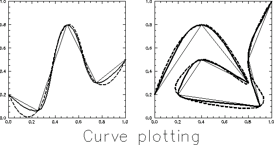
Figure
1. Curves generated by example program ZXCURV.
Example 2
������ PROGRAM ZXCHAR
C
C Example of character plotting.
C
������ CALL XDEVIC
������ CALL XPSPAC(0.1,0.9,0.1,0.9)
C
C Define a device reference point and the rotating angle
C of whole plot around the point.
������ CALL XDREFP(0.5,0.5)
C
C Map the picuture space.
������ CALL XMAP� (0.0,10.,0.0,1.0)
������ CALL XBORDR
������ CALL XCFONT(3)
C
C Plot character strings spanning over the x-picture space.
������ DIST=XPNTSD(0.0,0.0, 10.0,0.0)
������ CALL XCHMAG(DIST/XCHLEN('This is zxplot test'))
������ CALL XCHARR( 10.,0.15, 'This is zxplot test')
������ CALL XCHMAG(DIST/XCHLEN('ZXPLOT') )
������ CALL XCHARL( 0.0,0.7 , 'ZXPLOT')
C
������ CALL XCHMAG( 0.05 )
C
������ CALL XCFONT(4)
C
C Plot left, centered or right justified charater strings
C with underline and rotation options.
������ CALL XCHLIN(2)
������ CALL XCHARC( 5.0,0.5 , 'CENTER')
������ CALL XCHLIN(0)
������ CALL XCHORI( 45.0 )
������ CALL XCHARC( 5.0,0.35,'rotate' )
������ CALL XCHORI( 0.0 )
������ CALL XCFONT(2)
������ DO 4 J=0,6
������ CALL XCHMAG( .01+J*0.004)
������ CALL XCHARL(0.1, 0.3+J*.05,'Left justification')
�4���� CALL XCHARR(10., 0.3+J*.05, 'Right justification')
������ CALL XGREND
������ STOP
������ END

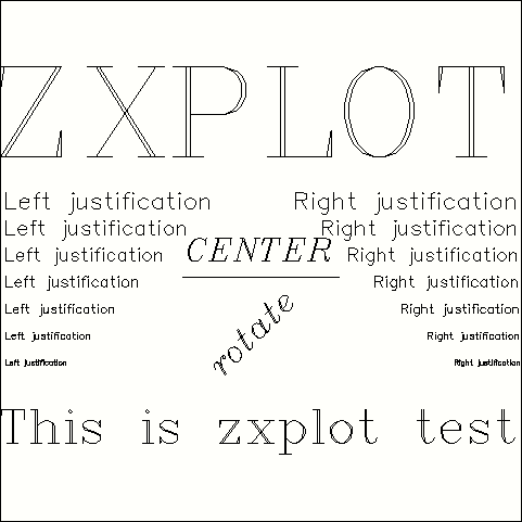
Figure 2. Sample character plotting
generated by program ZXCHARACTER.
Example 3
����� PROGRAM ZXTRAN
C
C This program demonstrates the use of coordinate transformations.
C
C Setup device and initialize ZXPLOT.
����� CALL XDEVIC
C
C Define a picture space.
����� CALL XPSPAC(0.1,0.9,0.1,0.9)
C
C Define a user coordinate on the picture space
����� CALL XMAP(0.0, 1.0,0.0,1.0)
����� call xthick(1)
C
����� CALL XAXFMT('(F3.1)')
����� CALL XAXES (0.0,0.0,0.0,0.0)
����� CALL XBORDR
����� call xthick(2)
C
C Set the reference point for coordinate transformation.
����� CALL XMREFP(0.0,0.0)
C
C To plot a quadratic curve.
����� A=0.1
����� B=0.05
����� CALL XPENUP(0.0,0.0)
����� DO� 5 I=1,50
������� X0=I/50.0
������� Y0=2.8*( 0.25-(X0-0.5)**2 )
������� CALL XPENDN(X0,Y0)
� 5�� CONTINUE
C
C����������������������� lot a series of ellipses along the curve.
����� DO 10 I=0,5
������� X0=I*0.2
������� Y0=2.8*( 0.25-(X0-0.5)**2 )
������� AK=-5.6*(X0-0.5)
������� ANG=180/3.14159*ATAN(AK)
C
C Shift the reference point to location (X0,Y0) and rotate piture
C through angle ANG.
������� CALL XMLOCA(X0,Y0)
���� ���CALL XMRANG(ANG)
������� CALL ELLIPS(0.0,0.0,A,B)
�10�� CONTINUE
����� CALL XMROFF
C
C Terminate graphics plotting.
�555� CALL XGREND
����� STOP
����� END
C
����� SUBROUTINE ELLIPS(X0,Y0,A,B)
C
C This subroutine draws an ellipse
C
����� PI=4*ATAN(1.0)
����� CALL XPENUP(X0+A,Y0)
����� DO 10 I=1,36
������� X=X0+A*COS(2*PI*I/36.0)
������� Y=Y0+B*SIN(2*PI*I/36.0)
������� CALL XPENDN(X,Y)
�10�� CONTINUE
����� CALL XPENUP(X0-A,Y0)
����� CALL XPENDN(X0+A,Y0)
����� CALL XPENUP(X0,Y0-B)
����� CALL XPENDN(X0,Y0+B)
����� RETURN
����� END

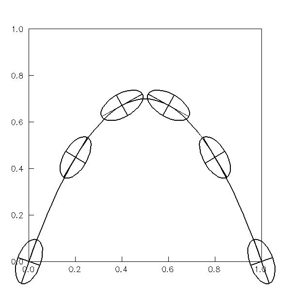
Figure 3. Example demonstrating
coordiante transform utilities in ZXPLOT.
Example 4
����� PROGRAM
ZXCONTOUR
C
C Example of contouring and color fill routines.
C
����� PARAMETER( M=31, N=21)
����� REAL Z(M,N),X(M,N),Y(M,N),CL(100)
����� INTEGER IW(M,N)
����� real xw(8*m), yw(8*m)
����� real xscale, yscale
�
����� xscale = 20.0
����� yscale = 10.0
����� DO 10 J=1,N
����� DO 10 I=1,M
������� Z(I,J)= SIN( I*2.0/M *3)*EXP( J*3.0/50)
������� X(I,J)= (0.01+(I-1.0)/(M-1)*0.98)*xscale
������� Y(I,J)= (0.01+(J-1.0)/(N-1)*0.98)*yscale
10��� CONTINUE
C
C Setup device and define plotting space.
c
����� call xpsfn('zxcont'//'.ps', 5)� ! PS output will be called zxout.ps
����� CALL XDEVIC
����� CALL XPSPAC(0.1,0.9,0.2,0.8)
����� CALL XMAP� (0.0,xscale,0.0,yscale) ! Define use plotting space
����� CALL XLABMASK(1)
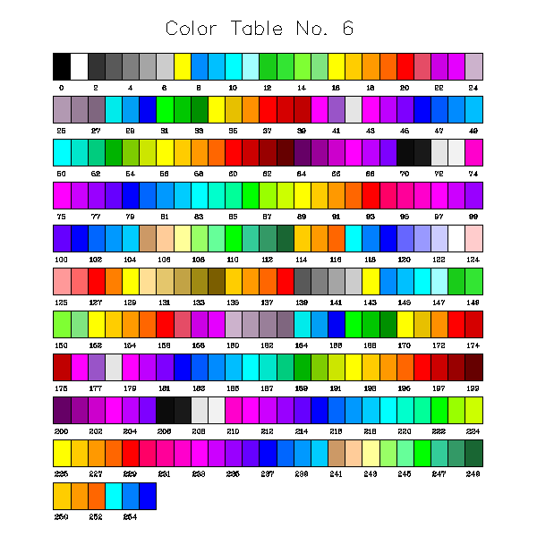
����� call xsetclrs(6)� ! Use internally defined color map number 6
����� call xcolor(1)��� ! Set color to black
����� call xcfont(3)
C
C Plot axes and labels
c
����� XSTEP=0.01*xscale
����� YSTEP=0.01*yscale
����� CALL XAXSCA(0.0,xscale,XSTEP,0.0,yscale,YSTEP)
C
C Set tentative color interval and limit on the min/max number of contours
c
����� CL(1)=0.0
����� CL(2)=0.20��������� ! Set tentative contour interval
����� call xnctrs(2,100)� ! Set lower and upper limits
������������������������� ! on the number of contours allowed
�������������� �����������! It's used by both xcolfil and xclimit
����� call xnctrs(2,30)� ! Set lower and upper limits
����� MODE=1
c���� z(2,3)=-9999.9
c���� call xctrbadv(1)�� ! Turn on bad value checking in contouring routine
c���� call xbadval( -9999.0 ) ! Specify bad value flag
c
c plot a color filled contour field for positive values
c
����� call xctrclr(10,39)������� ! Use colors between 10 and 39 inclusive
����� call xctrlim(0.0, -9999.0) ! Only contours above zero are plotted
����� call xctrlim(0.0, 0.0) ! Only contours above zero are plotted
����� CALL XColfil(Z(1,1),X,Y,IW,xw,yw,M,M,N, CL, NCL,MODE)
����� call xchsiz(0.02* yscale)� ! Set character size
����� call xcpalet(1)����������� ! Plot horizontal color palette
c���� call xcpalet(2)����������� ! Plot vertical�� color palette
c
c plot contours for negative values
c
����� call xhlfrq(1)� ! All contours are highlighted as thick lines
����� call xctrclr(185,208) ! Use colors between 185 and 208 inclusive
����� call xctrlim(-9999.0, 0.0) ! Only contours below zero are plotted
����� call xctrlim(0.0, 0.0) ! Only contours below zero are plotted
����� CALL XCONTA(Z(1,1),X,Y,IW,M,M,N, CL, NCL,MODE) ! Draw negative contours
����� ZMAX=CL(NCL)
����� ZMIN=CL(1)
����� ZINC=CL( MIN(2,NCL) )-CL(1)
����� CALL XCLIMT(ZMAX,ZMIN,ZINC,0.025*yscale) ! Write max/min limits
����� CALL XGREND� ! End graphics
����� STOP
����� END

Figure 4. Contour and color filled
fileds creted by example program ZXCONTOUR.
Example 5
����� PROGRAM
ZXHATCH
C
C Example of cross-hatching routines.
C
����� implicit none
����� integer m,n
����� PARAMETER( M=21, N=31)
c���� PARAMETER( M=6, N=6)
����� REAL Z(M,N),X(M,N),Y(M,N),CL(100)
����� INTEGER IW(M,N)
����� real xwk(m,n),ywk(m,n)
����� integer ncl,mode,i,j,k
����� real xstep,ystep,zmin,zmax,zinc,cl1,cl2
����� real xscale,yscale
����� real hx(m),hy(n)
����� real hx1(m),hy1(n)
C
����� xscale = 5.0
����� yscale = 10.0
����� DO 10 J=1,N
����� DO 10 I=1,M
������� Z(I,J)= SIN( 4.00*float(I*j)/(m*n))
������� X(I,J)= (I-1.0)/(M-1) * xscale
������� Y(I,J)= (J-1.0)/(N-1) * yscale
������� hx(i)= sin( 2*3.14*x(i,j)/xscale)*0.1*yscale
������� hy(i)= cos( 2*3.14*y(i,j)/yscale)*0.1*xscale
������� hx1(i)= yscale-sin( 2*3.14*x(i,j)/xscale)*0.05*yscale
� ������hy1(i)= xscale+cos( 2*3.14*y(i,j)/yscale)*0.05*xscale
������� y(i,j)= (y(i,j)-hx(i))/(hx1(i)-hx(i))*yscale
������� x(i,j)= (x(i,j)-hy(i))/(hy1(i)-hy(i))*xscale
10��� CONTINUE
�
C Setup device and define plotting space.
����� call xpsfn( 'zxhatch.ps' )
����� CALL XDEVIC
����� CALL XPSPAC(0.1,0.9,0.1,0.9)
����� CALL XMAP� (0.0,xscale,0.0,yscale)
C
C Draw a border and plot ticks and labels on the border.
c
����� XSTEP=0.05 * xscale
����� YSTEP=0.05 * yscale
C
C Call XCONTA and XCLIMT to plot a contour map with default options.
c
����� CL(1)=0.0
����� CL(2)=0.10
����� call xnctrs(2,100)
����� MODE=1
����� call xhlfrq(4)
����� call xhilit(0)
����� call Xcfont(3)
����� call xthick(2)
����� do j=1,n
������� call xpenup(x(1,j),y(1,j))
������� do i=2,m
������� call xpendn(x(i,j),y(i,j))
������� enddo
����� enddo
����� do i=1,m
������� call xpenup(x(i,1),y(i,1))
������� do j=2,n
������� call xpendn(x(i,j),y(i,j))
������� enddo
����� enddo
����� call xthick(1)
����� call xhllabl(1)
����� CALL XCONTA(Z(1,1),X,Y,IW,M,M,N, CL, NCL,MODE)
C
C Plot vertical hatching between contours
c
����� CALL XDHTCH(0.007)
����� cl(ncl+1)=cl(ncl)+zinc
����� DO 20 K=1,NCL,2
������� CL1=CL(K)
������� CL2=CL(K+1)
������� CALL XHATCHA(Z(1,1),X(1,1),Y(1,1),xwk,ywk,M,M,N,
���� :�� ����CL1,CL2,45.0)
������� CALL XHATCHA(Z(1,1),X(1,1),Y(1,1),xwk,ywk,M,M,N,
���� :������ CL1,CL2,-45.0)
�20�� CONTINUE
145�� CALL XGREND
����� STOP
����� END

Figure 5. Example plots of cross-hatched
contours. Also shown are plots of H at maximum locations.
Example 6.
����� PROGRAM
ZXVECTOR
C
C This program demonstrates the plotting of vector fields.
C
����� PARAMETER( M=20, N=20)
����� REAL X(M,N),Y(M,N),Z(M,N),U(M,N),V(M,N)
����� XSCALE=10.0
����� YSCALE=10.0
����� X0=0.5*XSCALE
����� Y0=0.5*YSCALE
����� XS=0.05*XSCALE
����� YS=0.05*YSCALE
����� DO 5 J=1,N
������� DO 5 I=1,M
��������� X(I,J)= (I-1.0)/(M-1.)*XSCALE
��������� Y(I,J)= (J-1.0)/(N-1.)*YSCALE
��������� Z(I,J)=( (X(I,J)-X0)/XS)**2- ( (Y(I,J)-Y0)/YS)**2
��������� V(I,J)=� (2*(X(I,J)-X0)/XS**2)/10 *6
��������� U(I,J)=� (2*(Y(I,J)-Y0)/YS**2)/10 *6
c�������� V(I,J)=� .0
c�������� U(I,J)=� 25.0
�5��� CONTINUE
����� CALL XDEVIC
����� CALL XPSPAC( 0.2,0.8, 0.05,0.45 )
����� CALL XMAP(0.0,XSCALE, 0., YSCALE )
����� CALL XAXSCA( 0.0, XSCALE, 0.1, 0.0, YSCALE, 0.1 )
� ����UUNIT=20.0
c���� UUNIT=5.0
����� ISTEP=1
����� JSTEP=1
C
C Determine the scale of vectors.
����� CALL XVECTU(U,V, M,M,ISTEP,N,JSTEP,XLENG,UUNIT)
c���� XLENG=0.8*XLENG
����� XLENG=1.5*XLENG
����� uunit = 15.0
����� xleng = xscale/(m-1)
C
C Plot vector fields and key vectors.
c
����� call XARTYP(2)
����� CALL XVECTR(U,V,X,Y,M,M,ISTEP,N,JSTEP,XLENG,UUNIT)
����� call xqmap(x1,x2,y1,y2)
����� call xchsiz( (y2-y1)*0.025 )
����� CALL XVECTK(-0.1*XSCALE,-0.1*YSCALE, XLENG, UUNIT,0)
����� call xchsiz( (y2-y1)*0.040 )
����� CALL XVLIMIT((x1+x2)*0.5,y2+0.03*(y2-y1),
���� :������������ 'Umax','Umin','Vmax','Vmin')
����� CALL XCHSIZ(0.05*(y2-y1))
����� CALL XCHARC(0.5*(x2+x1),y1-0.1*(y2-y1),'Vector field')
����� CALL XPSPAC( 0.2,0.8, 0.55,0.95 )
����� CALL XMAP(0.0,XSCALE, 0., YSCALE )
����� CALL XAXSCA( 0.0, XSCALE, 0.1, 0.0, YSCALE, 0.1 )
����� CALL XBARBS(U,V,X,Y,M,M,ISTEP,N,JSTEP,1,XLENG,1)
�
����� CALL XGREND
����� STOP
����� END

Figure 6. Example plots of vector
fields produced by program ZXVECTOR.
Example 7
PROGRAM ZXSURF
C
C Example for 3-D surface viewing (see Section 10)
C
����� PARAMETER (M= 40, N= 40)
����� REAL SURFAS(M ,N ),WORK(2*N)
C
C Generating datum surface
����� DO 100 I = 1, M
�������� X1=0.5*(I-10)
�������� DO 200� J = 1, N
����������� Y1=0.5*(J-25)
����������� R1= SQRT(X1*X1+Y1*Y1)
����������� T1=-1.0
����������� IF(ABS(R1).GT.1.E-5) T1=-SIN(R1)/R1
����������� SURFAS(I,J)=T1
� 200��� CONTINUE
� 100 CONTINUE
C
C Initiate ZXPLOT
����� CALL XDEVIC
C
C Set ploting space
����� CALL XDSPAC(1.0)
����� CALL XSPACE(1,3,0.0,XLIM,YLIM)
C
C To get a proportional space in x,y directions.
����� RATIO=YLIM/XLIM
����� CALL XMAP(-3.0 ,3.0 ,-3.0*RATIO,3.0*RATIO)
C
C Set character font and charater size.
����� CALL XCFONT(3)
����� CALL XCHMAG(0.02)
����� DO 10 K=2,4
������� CALL XNWPIC
������� CALL ZSFVEW( 5-K )
������� CALL ZSFANG(40.+(5-K)*20.)
������� CALL ZSFLOC(0.0,1.8-0.6*K,4.)
������� CALL ZSFPLT(SURFAS,M ,M ,N ,WORK)
������� CALL XCHARL(-2.,-1.0,'ZXPLOT example')
������� CALL XINUMB(0.5 ,-1.0, 5-K ,'(''IQS'',I2)' )
������� CALL XRNUMB(1.2,-1.0,40.+(5-K)*20.,'(''ANGLE'',F6.1)')
�10�� CONTINUE
����� CALL XGREND
����� STOP
����� END

Figure 7. 3D view of 2D surfaces.
Example 8
�����
PROGRAM ZXVIEW
C
C Example to demonstrate the 'special effects' through combined use
C of coordinate transformations and user-defined projection.
C
����� PARAMETER( M=20, N=20)
����� REAL U(M,N),V(M,N),X(M,N),Y(M,N),Z(M,N),CL(100)
����� INTEGER IW(M,N)
����� XSCALE=1.0
����� YSCALE=1.0
����� X0=0.5*XSCALE
����� Y0=0.5*YSCALE
����� XS=0.05*XSCALE
����� YS=0.05*YSCALE
����� DO 5 J=1,N
������� DO 5 I=1,M
��������� X(I,J)= (I-1.0)/(M-1.)*XSCALE
��������� Y(I,J)= (J-1.0)/(N-1.)*YSCALE
��������� Z(I,J)=-(X(I,J)-X0)*(Y(I,J)-Y0)/(XS**2)
��������� V(I,J)=-(Y(I,J)-Y0)/(XS*XS)
��������� U(I,J)= (X(I,J)-X0)/(XS*XS)
�5��� CONTINUE
����� CALL XDEVIC
����� CALL XDSPAC(0.9)
����� CALL XPSPAC( 0.3,0.9 , 0.0,0.3)
����� CALL XMAP(0.0,XSCALE, 0.0,YSCALE )
����� CALL XMREFP(0.0,0.0)
C
C Project Cartesian space onto a 'perspective' space.
����� CALL XPRJON
����� CALL XOBANG( 15.0, 45.0 )
C
C Calculate contour values and determine unit vector length.
����� ZINC=0.5
����� CALL XCLEVL(Z,M,M,N,ZMAX,ZMIN,ZINC,CL,NCNT)
����� UUNIT=5.0
����� ISTEP=1
����� JSTEP=1
����� CALL XVECTU(U,V, M,M,ISTEP,N,JSTEP,XLENG,UUNIT)
����� XLENG=0.8*XLENG
����� CALL XCLTYP(0)
����� CALL XDREFP(0.4, 0.0)
����� CALL XOBANG( 20.0, 45.0 )
����� CALL XBORDR
����� CALL XVECTR(U,V,X,Y,M,M,ISTEP,N,JSTEP,XLENG,UUNIT)
C
����� CALL XDLOCA(0.4,0.35)
����� CALL XOBANG( 15.0, 45.0 )
����� CALL XBORDR
����� CALL XCONTA(Z,X,Y,IW,M,M,N,CL,NCNT,3)
C
����� CALL XDLOCA(0.4,0.7)
����� CALL XOBANG( 10.0, 45.0 )
����� CALL XBORDR
����� CALL XVECTR(U,V,X,Y,M,M,ISTEP,N,JSTEP,XLENG,UUNIT)
C
C Cancel transformations.
����� CALL XUNDLC
����� CALL XPRJOF
����� CALL XGREND
����� STOP
����� END
c���� SUBROUTINE XPROJC(X,Y)
c���� PARAMETER (PI05=3.1415926535*0.5 , PI05DR=PI05/90 )
c���� PARAMETER (ALPHA= 20.0*PI05DR, BELTA=-8*PI05DR )
C Alpha / Belta -- the rotation angle of the right /top edge of each
C picture ( before any transformation ) relative to y-axis / x-axis.
c���� CALL XQMAP(XL,XR,YB,YT)
c���� XL=XLTRNX( XL)
c���� XR=XLTRNX( XR)
c���� YB=XLTRNY( YB)
c���� YT=XLTRNY( YT)
c���� X1=XLTRNX( X )
c���� Y1=XLTRNY( Y )
c���� XANG=ALPHA*(X1-XL)/(XR-XL)
c���� YANG=BELTA*(Y1-YB)/(YT-YB)
c���� XK=-TAN( XANG )
c���� YK= TAN( YANG )
c���� DEN=1-XK*YK
c���� X=(X1+XK*(Y1-YB-YK*XL))/DEN
c���� Y=(Y1+YK*(X1-XL-XK*YB))/DEN
c���� CALL XLINVT(X,Y)
c���� RETURN
c���� END

Figure 8. 3D
perspective views of 2D planes at different levels.
Example 9
ZXMAP.f file:
����� PROGRAM
ZXMAP
c
c���� Program to plot rectangular grids in a map projection space
c���� with map lines.
c����
c���� Commands:
c�
c���� zxncarf77 -o zxmap zxmap.f
c or� zxpostf77 -o zxmap zxmap.f
c
c���� zxmap < zxmap.input
c
����� implicit none
����� integer mapproj
����� real dx,dy,ctrlat,ctrlon,trulat1,trulat2,trulon,sclfct,xl,yl
����� integer nx,ny
����� namelist /grid/ nx,ny,dx,dy,ctrlat,ctrlon
����� namelist /projection/ mapproj,trulat1,trulat2,trulon,sclfct
����� integer nnestgrid,nxng(20),nyng(20)
����� real xctrng(20),yctrng(20),dxng(20),dyng(20)���
����� namelist /newgrid/nnestgrid,nxng,nyng,xctrng,yctrng,dxng,dyng
����� integer ovrmap,nmapfile,lmapfile,i, mxmapfile
����� parameter (mxmapfile= 10)
����� character mapfile(mxmapfile)*132
����� namelist /map_plot/ovrmap,latgrid,longrid,nmapfile,mapfile
����� logical fexist
����� real xl1, yl1, ctrlat1, ctrlon1
����� real latgrid,longrid,xorig,yorig
c
C@@@@@@@@@@@@@@@@@@@@@@@@@@@@@@@@@@@@@@@@@@@@@@@@@@@@@@@@@@@@@@@@@@@@@@@
C
C���� Beginning of executable code...
C
C@@@@@@@@@@@@@@@@@@@@@@@@@@@@@@@@@@@@@@@@@@@@@@@@@@@@@@@@@@@@@@@@@@@@@@@
c
c
c#######################################################################
c
c���� Input control parameters map plotting
c
c#######################################################################
c
����� write(6,'(/a/)')
���� :' Please input control parameters for map plotting.'
����� read(5,grid,err=100)
����� write(6,'(1x,a,i8)')'Input nx was',nx
����� write(6,'(1x,a,i8)')'Input ny was',ny
����� write(6,'(1x,a,f10.3,a)')'Input dx was',dx,' meters'
����� write(6,'(1x,a,f10.3,a)')'Input dy was',dy,' meters'
����� write(6,'(1x,a,f10.3,a)')
���� :���� 'Input ctrlat was ',ctrlat,' degree North'
����� write(6,'(1x,a,f10.3,a)')
���� :���� 'Input ctrlon was ',ctrlon,' degree East'
C#######################################################################
c
c���� Input map projection parameters
c
C#######################################################################
c
����� READ (5,projection,err=100)
�� ���write(6,'(1x,a,i4)') 'Input mapproj was ',mapproj
����� write(6,'(1x,a,f10.3,a)')
���� :���� 'Input trulat1 was ',trulat1,' degree North'
����� write(6,'(1x,a,f10.3,a)')
���� :���� 'Input trulat2 was ',trulat2,' degree North'
����� write(6,'(1x,a,f10.3)')
���� :� 'The latitude of the center of the model domain was ',ctrlat
����� write(6,'(1x,a,f10.3)')
���� :� 'The longitude of the center of the model domain was ',ctrlon
����� write(6,'(1x,a,f10.3,a)')
���� :���� 'Input trulon was ',trulon,' degree East'
����� IF ( mapproj .eq. 0 ) THEN
������� trulat1 = ctrlat
������� trulat2 = ctrlat
������� trulon� = ctrlon
����� ENDIF
c
c#######################################################################
c
c���� Set the output grid and the variable control parameters
c
c#######################################################################
c
����� READ (5,newgrid)
����� write(6,'(1x,a,i2)') 'Input nnestgrid was ',nnestgrid
����� DO i=1,nnestgrid
������� write(6,'(1x,a,i2.2,a,i5)�� ')'Input nxng(',i,')� =',nxng(i)
������� write(6,'(1x,a,i2.2,a,i5)�� ')'Input nyng(',i,')� =',nyng(i)
������� write(6,'(1x,a,i2.2,a,f15.3)')'Input dxng(',i,')� =',dxng(i)
������� write(6,'(1x,a,i2.2,a,f15.3)')'Input dyng(',i,')� =',dyng(i)
������� write(6,'(1x,a,i2.2,a,f15.3)')'Input xctrng(',i,')=',xctrng(i)
������� write(6,'(1x,a,i2.2,a,f15.3)')'Input yctrng(',i,')=',yctrng(i)
����� ENDDO
����� read(5,map_plot,err=100)
����� write(6,'(1x,a,i2)')'Input ovrmap =',ovrmap
����� write(6,'(1x,a,f10.3)') 'Input latgrid=',latgrid
��� ��write(6,'(1x,a,f10.3)') 'Input longrid=',longrid
����� write(6,'(1x,a,i2)')'Input nmapfile=',nmapfile
����� DO i=1,min(mxmapfile,nmapfile)
������� write(6,'(1x,a,i2.2,a,a)')'Input mapfile(',i,') =',mapfile(i)
����� enddo
����� write(6,'(/)')
����� GOTO 10
100�� write(6,'(a)') 'Error reading NAMELIST file. Program stopped.'
����� stop
10��� CONTINUE
c
c#######################################################################
c
c���� Initialize ZXPLOT plotting package
c
c#######################################################################
c
����� CALL xdevic
����� CALL setcolors(1)
����� CALL xcolor(1)
����� CALL xartyp(2)
����� CALL xdspac(0.9)
����� CALL xaxfmt( '(i10)' )
c#######################################################################
c
c���� Set map
c
c#######################################################################
c
����� xl = (nx-3)*dx * 0.001
����� yl = (ny-3)*dy * 0.001
����� xorig = 0.0
����� yorig = 0.0
����� CALL XSTPJGRD(mapproj,trulat1,trulat2,trulon,
���� :����������� ��ctrlat,ctrlon,xl,yl,xorig,yorig)
����� if( xl.ge.yl) then
������� call xpspac(0.1,0.9, 0.5-yl/xl*0.4,0.5+yl/xl*0.4)
����� else
������� call xpspac(0.5-xl/yl*0.4,0.5+xl/yl*0.4,0.1, 0.9)
����� endif
c
����� CALL xmap(0.0,xl, 0.0, yl)
����� CALL xaxsca(0.0,xl, dx/1000.0, 0.0, yl, dy/1000.0 )�
����� call xthick(3)
����� CALL xcolor(6)
����� DO 500 i=1,nnestgrid
������� xl1 = (nxng(i)-3)*dxng(i) * 0.001
������� yl1 = (nyng(i)-3)*dyng(i) * 0.001
������� CALL xbox(xctrng(i)*0.001-xl1/2,xctrng(i)*0.001+xl1/2,
���� :����������� yctrng(i)*0.001-yl1/2,yctrng(i)*0.001+yl1/2)�
500�� CONTINUE
����� CALL xcolor(1)
����� call xthick(1)
����� call xcolor(9)
����� IF( ovrmap .ne.0 ) then
�
������� DO 700 i=1,min(mxmapfile,nmapfile)
�
������� lmapfile=132
������� CALL xstrlnth(mapfile(i), lmapfile)
c������ write(6,'(1x,a,a)') 'Input was ',mapfile(i)(1:lmapfile)
�
������� INQUIRE(file=mapfile(i)(1:lmapfile), exist = fexist )
������� IF( .not.fexist) THEN
��������� write(6,'(a)') 'Map file '//mapfile(i)(1:lmapfile)//
���� :��� ' not found. Corresponding map no plotted.'
������� ELSE
��������� call xthick(1)
��������� if( i.eq.1) call xthick(2)
��������� call xdrawmap(10,mapfile(i)(1:lmapfile),latgrid,longrid)
������� ENDIF
�
700���� CONTINUE
�
����� ENDIF
����� call xthick(1)
����� DO i=1,nnestgrid
������� CALL xxytoll(1,1,xctrng(i),yctrng(i),ctrlat1,ctrlon1)
������� write(6,'(/1x,a,i2,a,/1x,a,2(f14.3,a),2(f9.4,a))')
���� :� 'For nested grid number ',i,',',
���� :� 'xctr,yctr,ctrlat,ctrlon=',
���� :� xctrng(i),',',yctrng(i),',',ctrlat1,',',ctrlon1,'.'
����� ENDDO
����� CALL xframe
800�� CALL xgrend
����� STOP
����� END
zxmap.input file:
c
c
c#######################################################################
c
c� This file contains the input parameters in namelist format for
c� program ZXMAP.
c
c� Steps to use this program:
c�
c� Step 1: Compile and link using 'zxncarf77 -o zxmap zxmap.f'
c� Step 2: Edit input file zxmap.input
c� Step 3: Run job using 'zxmap < zxmap.input'.
c
c#######################################################################
c
c�� Author:
c
c�� Ming Xue (03/27/1997)
c
c#######################################################################
c
c� nx������ Number of grid points in x direction.
c� ny������ Number of grid points in y direction.
c
c� dx������ Grid spacing in x-direction in computational
c���������� and physical space (m).
c� dy������ Grid spacing in y-direction in computational
c���������� and physical space (m).
c
c� ctrlat�� Latitude of the model physical domain center (deg. N).
c� ctrlon�� Longitude of the model physical domain center (deg. E).
c
c#######################################################################
�&grid
�� nx���� =� 171,
�� ny��� �=� 171,
�� dx���� =� 6000.000,
�� dy���� =� 6000.000,
�� ctrlat =��� 34.0000,
�� ctrlon =� -97.00,
�&END
c#######################################################################
c
c� Projection parameters:
c
c� mapproj�� Map projection option.
c�������� �= 0, no map projection;
c��������� = 1, polar projection;
c��������� = 2, Lambert projection;
c��������� = 3, Mercator projection.
c� trulat1�� 1st true latitude of map projection.
c� trulat2�� 2nd true latitude of map projection (used only by mapproj =
2).
c� trulon��� True longitude of map projection.
c
c#######################################################################
�&projection
�� mapproj = 2,
�� trulat1 =� 30.0,
�� trulat2 =� 50.0,
�� trulon� = -100.0,
�� sclfct� =� 1.0,
�&END
c#######################################################################
c
c� There are parameters for another grid box grid.
c
c� nnestgrid� Number of nest grid boxes to draw. Maxmum = 20
c� nxng������ Number of grid points in x-direction for the nested grid(s).
c� nyng������ Number of grid points in y-direction for the nested grid(s).
c
c� dxng������ Grid interval of the nested grid(s). in x direction.
c� dyng������ Grid interval of the nested grid(s). in y direction.
c
c� xctrng���� x-coordinate of the center of nested grid(s).
c� yctrng���� y-coordinate of the center of nested grid(s).
c
c#######################################################################
�&newgrid
�� nnestgrid = 1,
�� nxng(1)�� = 195,
�� nyng(1)�� = 135,
�� dxng(1)�� = 3000.0,
�� dyng(1)�� = 3000.0,
�� xctrng(1) =� 600000.0,
�� yctrng(1) =� 650000.0,
�&END
c
c#######################################################################
c
c� ovrmap� Option to overlay political map on horizontal plane plots
c��������������� = 0, no map overlay.
c���� �����������= 1, overlay map on all of the ploted fields.
c
c� latgrid,longrid (degree)
c������������ the intervals between lat and lon grid lines.
c������������ < 0.0, no grid lines in the given direction,
c������������ = 0.0, internally determined,
c���� ��������= any real number, typically from 1.0 to 10.0 degrees.
c� nmapfile�� number of mapfiles ( maximum=2)
c� mapfile��� Mapdata file name.
c
c#######################################################################
c
�
�&map_plot
�� ovrmap = 1,
�� latgrid = 10.,
�� longrid = 10.,
�� nmapfile = 2,
���� mapfile(1) = '../data/us_state.mapdata',
���� mapfile(2) = '../data/us_spcounty.mapdata',
�&END

Figure 9. State and counter map
lines in the southern plain of US, using Lambert projection.
Example 10
The following is a list of application subroutines of section 11. They
also serve as examples of the use of ZXPLOT. The inclusion of these
subroutines in user's program will overwrite the equivalence in ZXPLOT
library.
���� SUBROUTINE XCONTS(Z,X,Y,MD,ND, ZINC)
���� REAL Z(MD,ND),X(MD,ND),Y(MD,ND),CL(150)
���� INTEGER IWRK(10000)
���� CL(1)=0.0
���� CL(2)=ZINC
���� MODE=1
���� M =MD
���� N =ND
���� IST=1
���� JST=1
���� CALL XCONTA(Z(IST,JST),X(IST,JST),Y(IST,JST)
����: ,IWRK,MD,M,N,CL,NCL,MODE)
���� ZMAX =CL(NCL)
���� ZMIN =CL( 1)
���� ZINC1=CL(MIN(2,NCL))
���� CALL XCLIMT(ZMAX,ZMIN,ZINC1,0.0)
���� RETURN
���� END
SUBROUTINE XCLIMT(FMAX,FMIN,FINC )
CHARACTER CH*150
CALL XQMAP(XL,XR,YB,YT)
CALL XQRANG( XRG, YRG )
CALL XQCHMG( SIZ0 )
SIZ=0.04*MIN( XRG, YRG)
CALL XCHMAG(SIZ)
WRITE(CH,'(''Min='',G9.3E2,'' Max='',G9.3E2,
: '' Contour interval='',G9.3E2)')FMIN,FMAX,FINC
CALL XCHARC( 0.5*(XL+XR), YT+0.03*(YT-YB),CH(1:54) )
CALL XCHMAG( SIZ0)
RETURN
END
SUBROUTINE XVECTS(U,V,X,Y,MD,ISTEP,ND,JSTEP,XLENG1,UUNIT1)
REAL U(MD,ND),V(MD,ND),X(MD,ND),Y(MD,ND)
M =MD
N =ND
IST=1
JST=1
XLENG=XLENG1
UUNIT=UUNIT1
CALL XVECTU(U(IST,JST),V(IST,JST),MD,M,ISTEP,N,JSTEP,XLENG,UUNIT)
CALL XVECTR(U(IST,JST),V(IST,JST),X(IST,JST),Y(IST,JST),
: MD,M,ISTEP,N,JSTEP,XLENG,UUNIT)
CALL XQMAP(XL,XR,YB,YT)
X0=XL+(XR-XL)*0.75
Y0=YT+(YT-YB)*0.03
KEY=0
AM=1.0
IF( (M-1)/ISTEP.GT.30) AM=2.0
CALL XVECTK(X0,Y0,XLENG*AM,UUNIT*AM, KEY)
CALL XVLMT(0.0)
RETURN
END
SUBROUTINE XVLIMT(UMAX,UMIN,VMAX,VMIN )
CHARACTER CH*80
CALL XQMAP(XL,XR,YB,YT)
CALL XQCHMG( SIZ0 )
CALL XQRANG( XRG, YRG )
CALL XQCHMG( SIZ0 )
SIZ=0.04*MIN( XRG, YRG)
CALL XCHMAG(SIZ)
WRITE(CH,'('' Umax='',G9.3E2,'' Umin='',G9.3E2)')UMAX,UMIN
WRITE(CH(31:60),'('' Wmax='',G9.3E2,'' Wmin='',G9.3E2)')VMAX,VMIN
CALL XCHARL(XL,YT+0.03*(YT-YB),CH(31:60))
CALL XCHARL(XL,YT+0.08*(YT-YB),CH(1:30) )
CALL XCHMAG( SIZ0)
RETURN
END
SUBROUTINE XCAPTN(TITLES,NUM,CH,
LC )
C PLOT CAPTIONS ALONG THE BORDER
CHARACTER TITLES(NUM)*50, CH*100
CALL XQMAP(XL,XR,YB,YT)
CALL XQRANG( XRG, YRG )
CALL XQCHOR( ANG0 )
CALL XQCHMG( SIZ0 )
SIZ=0.05*MIN( XRG, YRG)
HX=SIZ*(XR-XL)/XRG
HY=SIZ*(YT-YB)/YRG
CALL XCHMAG( SIZ )
IF( NUM.GE.1) THEN
CALL XQOBAG( XANG, YANG )
CALL XCHORI( 90.0 +YANG-XANG )
CALL XCHARC( XL- 2.5*HX, 0.5*(YT+YB), TITLES(1)(1:10) )
CALL XCHORI(0.0)
CALL XCHARC( 0.5*(XR+XL), YB-2*HY , TITLES(1)(11:20))
ENDIF
IF( NUM.GE.2) THEN
CALL XCHARL(XL,YB-4*HY ,TITLES(2)(1:20))
CALL XQCPEN( XCP, YCP )
CALL XCHARL( XCP, YCP, ' '//CH(1:LC))
ENDIF
CALL XQCPEN( XCP, YCP )
YCP=YCP-0.5*HY
DO 10 K=3,NUM
CALL XCHARL(XL, YCP-HY , TITLES(K))
CALL XQCPEN( XCP, YCP )
10 CONTINUE
CALL XCHORI( ANG0 )
CALL XCHMAG( SIZ0 )
PRINT*, TITLES(2)(1:20) ,' is to be plotted..'
RETURN
END
13. Examples
of Color Table
The following color tables 1 through
6 are buildin in ZXPLOT, and can be plotted using program pltctable.f found
in examples directory. pltctable.f is listed here:
����� PROGRAM
pltctable
c
c This program plot a color table
c
����� implicit none
����� integer coltab
����� character coltabfn*80, ch*132
����� integer kcout, len
����� parameter(kcout=25)
����� integer i, num,� lind(kcout)
����� real cline(kcout)
����� real lblmag
����� common /labmag/ lblmag
����� integer icolor,lbcolor��������������� ! required color
����� common /recolor/icolor,lbcolor
����� real xl, xr, yb,yt
�����
����� lblmag=1.0
����� lbcolor=1
����� CALL xdevic
����� xl=0.10
����� xr=0.90
��� ��yb=0.01
����� yt=0.99
����� CALL xdspac(1.0)
����� CALL xwindw(xl, xr, yb, yt)
����� print*,'enter color table (-1 or 1 to 6)'
����� print*,'Enter 1 to 6 for ZXPLOT buildin color maps'
����� write(6,'(a,a)')' Enter -1 for your own color map.',
���� :� ��������������' You will need to give the file name'
����� read(5,*) coltab
����� IF(coltab.eq.-1) THEN
������� print*,'Please enter color file name (quote the name) '
������� read(5,*) coltabfn
������� CALL XSTCTFN(coltabfn)
������� len = index(coltabfn, ' ')-1
������� write(ch,'(''Color map file is: '',a)') coltabfn(1:len)
������� print*,'The color map file is:',coltabfn(1:len)
����� ELSE
������� write(ch,'(''Color Table No.'',i2)') coltab
����� ENDIF
����� CALL xsetclrs ( coltab )
����� CALL xcolor(lbcolor)
����� CALL xafstyl(1)
����� CALL xartyp(2)
����� call xhlfrq(20)
����� CALL xchsiz(0.035*(yt-yb)* lblmag )
����� IF(len.gt.50) CALL xchsiz(0.029*(yt-yb)* lblmag )
����� len = 132
����� CALL xstrmin(ch, len)
����� call xcharc(0.5, 0.935, ch(1:len))
����� CALL xchsiz(0.025*(yt-yb)* lblmag )
����� yb=0.85
����� yt=0.90
����� DO 45 num=0,9
������� DO i=1,kcout
��������� lind(i)= num*kcout+i-1
��������� cline(i) = float(num*kcout+i-1)
������� END DO
������� CALL LABEL(lind,cline,0.1,0.9,yb, yt ,kcout)
������� yb=yb-0.08
������� yt=yt-0.08
45��� CONTINUE
����� DO 50 i = 1,6
������� lind(i)= 249+i
������� cline(i) = float (249+i)
50��� CONTINUE
����� CALL LABEL(lind,cline,0.1,0.9,yb, yt ,6)
����� CALL xgrend
����� STOP
����� END
����� SUBROUTINE LABEL(lind,cline,xl,xr,yb,yt, kcolor)����������������
c
c Generate color label plots of 2-d field A given its
c coordinate using ZXPLOT and ncar package..
c
����� implicit none
����� integer k,l
����� integer kcout
����� parameter (kcout=25)
����� real xl,xr,yb,yt�� ! the physical domain space left, right, bottom,
top
����� integer lind(kcout)
����� character*20 llbs
����� character*20 ctmp
����� real xra(5),yra(5)���� ! array for single color box
����� real dtx
����� real x,y������������ ! color values position
����� real xs,ys
����� real cline(kcout)
����� real lblmag
����� common /labmag/ lblmag
����� integer icolor,lbcolor��������������� ! required color
����� common /recolor/icolor,lbcolor
����� integer kcolor
����� real xleft,xright
c
����� xs= xr-xl
�� ���ys= yt-yb
����� CALL xcfont(3)
����� CALL xchsiz(0.25*ys* lblmag )
����� dtx=xs/real(kcout)
����� y=yb-0.37*ys
����� DO 10 k=1,kcolor
������� xleft =xl+dtx*real(k-1)
������� xright=xl+dtx*real(k)
������� xra(1)=xleft
������� xra(2)=xright
������� xra(3)=xright
������� xra(4)=xleft
������� xra(5)=xleft
������� yra(1)=yt
������� yra(2)=yt
������� yra(3)=yb
������� yra(4)=yb
������� yra(5)=yt
������� CALL XCOLOR(lind(k))
������� call XFILAREA(xra,yra,5)
������� CALL xcolor(1)
������� call XBOX(xra(1),xra(2),yb,yt)
������� IF (kcout.lt.20 .or.
���� :��� (kcout.ge.20 .and. mod(k-1,2).eq.0) ) THEN
��������� CALL XRCH(cline(k),ctmp,l)
��������� llbs=ctmp(1:l-2)
��������� CALL color(lbcolor)
��������� x = (xra(1)+xra(2))*0.5
��������� CALL xcharc(x,y,llbs(1:l-2))
������� END IF
�10�� CONTINUE
����� CALL xcolor(lbcolor)
����� CALL xwdwof
����� RETURN
����� END


The following is one of the customer
made color maps, given as hubcaps5.pltcbar found in color_maps directory.
It is read in when color map option is set to -1. A customer color map is
created by listing RGB values in each line of an ASCII file. See hubcaps5.pltcbar
for example.

AN EXAMPLE OF ZXPLOT INTERFACE
with GKS.
There are only eight entries serving as interface routines in ZXPLOT. If
one wants to connect ZXPLOT with a new graphic system, the only work
needed is to build a similar interface following the example shown
below.
ZXPLOT interface with GKS, comforming to the NCAR GKS standard at level
0A. The subroutines in bold case called in the program are the GKS primitives.
SUBROUTINE XDEVIC
C
C* GKS OUTPUT PRIMITIVES
C* 1. POLYLINE GPL(N,X,Y)
C* 2. POLYMARKER GPM(N,X,Y)
C* 3. TEXT GTX(X,Y,STRING)
C* 4. FILL AREA GFA(N,X,Y)
C* 5. CELL ARRAY GCA(PX,PY,QX,QY,N,M,DIMX,COLIA)
C
C Set up divice
ierror=6
IFILE=2 ! channel for output CGM file.
CALL GOPKS(ierror,idummy)
CALL GOPWK(1,IFILE,1)
CALL GACWK(1)
C set default fill area style to hatch
CALL GSFAIS(3)
C set default hatch style to right slanting lines
CALL GSFASI(3)
C Initialization of this pachage
CALL XICHAR
CALL XDSPAC( 1.0 )
CALL XMINIT
RETURN
END
SUBROUTINE XDSPAC(PSIZE)
C
C Define a normalized device (ND) space (0.0,XSIDE,0.0,YSIDE) on device
C provided. The size of this space is 'PSIZE' times of the max device
C space. YSIDE should be 1.0, XSIDE can be bigger or smaller that 1.0
C depending on device.
C XSIDE, YSIDE should be passed to ZXPLOT through common block PSIDES.
C This routine sets up this space based on GKS.
C
COMMON /XPSIZE/ PSIZE1
COMMON /XPSD01/ XSIDE, YSIDE
PSIZE1=PSIZE
IF( PSIZE.LE.0.0) THEN
PRINT*,'ZERO OR NEGATIVE VALUES FOR PSIZE NOT PERMITTED!'
PRINT*,'IF SHOULD BE IN RANGE OF 0.1 TO 1.0,PLEASE RESET VALUE'
STOP
ENDIF
CALL GSCLIP(1) !Clipping is switched on for the defined view port.
CALL GSVP(1 , 0.0, 1.0, 0.0, 1.0) !Use the maximum device space.
XSIDE=1.0
YSIDE=1.0
EDGEX=0.5*XSIDE*(1.0/PSIZE-1)
EDGEY=EDGEX
X1=-EDGEX
X2= EDGEX+XSIDE
Y1=-EDGEY
Y2= EDGEY+YSIDE
CALL GSWN(1 , X1, X2, Y1,Y2)
CALL GSELNT(1 ) ! To activate the window-viewport mapping.
RETURN
END
SUBROUTINE XFRAME
C Advance plotting onto next frame
CALL XQMAP ( X1,X2,Y1,Y2 )
CALL XLPNUP(X1,Y1)
CALL GCLRWK( 1, 1)
RETURN
END
SUBROUTINE XGREND
C Terminate graphic plotting
CALL XQMAP ( X1,X2,Y1,Y2 )
CALL XLPNUP(X1,Y1)
CALL GDAWK( 1 )
CALL GCLWK( 1 )
CALL GCLKS
RETURN
END
SUBROUTINE PPENUP(X1,Y1)
DIMENSION XG(2),YG(2)
SAVE XG,YG
C Connect pen up routines
XG(1)=X1
YG(1)=Y1
RETURN
ENTRY PPENDN(X1,Y1)
C Connect pen down routines
XG(2)=X1
YG(2)=Y1
CALL GPL( 2, XG, YG )
XG(1)=X1
YG(1)=Y1
RETURN
END
SUBROUTINE ZFILLN(X,Y,NP)
C
C Fill area enclosed by (X(i),Y(i),i=1,NP) by a pre-specifeid
C pattern or colour index.
C Note that input X,Y represent the math coord.
C Whereas on exit X,Y are changed to ND coord.
C
REAL X(*),Y(*)
DO 100 I=1,NP
100 CALL XTRANS(X(I),Y(I))
C
C To link GKS fill area premitive.
C GSFAIS(INTS) should be called before to set the fill area style, where
C INTS=0 for hollow fill, =1 for solid fill, =2 for pattern fill and
C =3 for hatch fill.
C Then GSAFSI(istyle) can be called to set the hatch or pattern style.
C In NCAR graphics, hatch options are 1 for horizontal, 2 for vertical,
C 3 for right slanting, 4 for left slanting line, and 5 to horizontal and
C vertical lines, 6 for right and left slanting lines.
C
CALL GFA(NP,X,Y)
RETURN
END
Appendix A. List of entry names
CSAAAA XCLFMT XICH XPRJOF XSEAMQ
CSBBBB XCLFRQ XINUMB XPRJON XSHEAR
CSCCCC XCLIMT XLABEL XPROJC XSPACE
CSDDDD XCLTYP XLBFM XPSCAL XSROFF
DEC XCMIXL XLBINT XPSCOF XSRSET
ICLENG XCONTA XLBMAG XPSPAC XTHICK
XARROW XCONTR XLBOFF XQBRKN XTPNDN
XAXANT XCONTS XLBON XQCFNT XTPNUP
XAXES XCPNDN XLBROT XQCHLN XTRANS
XAXFMT XCPNUP XLBSIZ XQCHMG XUNDLC
XAXINC XCTRAN XLETER XQCHOB XUNMLC
XAXISX XCTREF XLINVT XQCHOR XVECTK
XAXISY XCURDN XLPNDN XQCHSZ XVECTR
XAXSCA XCURDV XLPNUP XQCPEN XVECTS
XAXTIK XCURUP XLTRNX XQCVMD XVECTU
XBORDR XCURVE XLTRNY XQDLOC XVLIMT
XBOX XCVMTD XMAP XQDRAG XVLMT
XBROKN XCZERO XMINIT XQDREF XVSCAL
XCAPTN XDASH XMLOCA XQFULL ZCONTA
XCDASH XDHTCH XMRANG XQLABL ZCONTB
XCDOT XDLOCA XMREFP XQLBON ZCONTC
XCFONT XDOT XMROFF XQMAP ZCONTM
XCFULL XDRANG XMRSET XQMLOC ZCONTR
XCHARC XDREFP XNCTRS XQMPEN ZQCONM
XCHARL XDROFF XNWFRM XQMRAG ZRCNTA
XCHARR XDRSET XNWPIC XQMREF ZRCNTB
XCHDEC XFULL XOBANG XQNPIC ZRCNTR
XCHLEN XGRAPH XOBOFF XQOBAG ZSFANG
XCHLIN XGRPDN XOBSET XQPPEN ZSFLOC
XCHLJ XGRPUP XPENDN XQPSCL ZSFPLT
XCHMAG XHATCH XPENUP XQPSPC ZSFSCL
XCHOBL XHATCX XPMAGN XQRANG ZSFSTL
XCHORI XHATCY XPNTSD XQTHIK ZSFVEW
XCHRST XHAT01 XPNTSZ XQUADR ZSF001
XCHSIZ XHILIT XPOINT XRCH ZSF002
XCLEVL XHLFRQ XPPONT XRNUMB ZSF003
----------------------------------------------------
The following are the interface routines
PPENDN XDEVIC XFRAME XICHAR
PPENUP XDSPAC XGREND ZFILLN
Appendix B. List of common
block names
XAGS09 XCHR31 XFTR06 XMAP04 XPRJ26
XASC12 XCHR32 XLAB14 XMRF08 XPSD01
XAXS18 XCIR25 XLAB15 XPEN11 XSCS10
XCDV23 XCLM19 XLAB16 XPHO03
XCHA20 XCMD24 XLPN13 XPHY01
XCHP21 XCRF17 XMAO05 XPRF07
Note : The common block names (the same as some entry and subroutine names)
are listed here in case of coincidence of names in users' programs.
Appendix C.
Index of subroutine entries in ZXPLOT
